How to filter by subtotals if over $5000 - Pivot Table/VBA?

[zander140]

Hello everyone, 

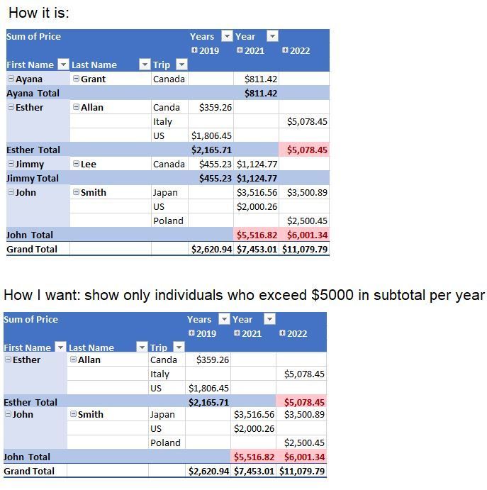
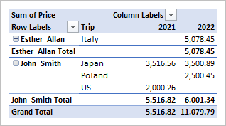
I was wondering in a Pivot Table, how can I filter/use a slicer to display all individuals who have a subtotal over $5000 per year. 

I did conditional formatting to identify such individuals (highlights subtotals in red) but the pivot table would not let me isolate them to show only the individuals with subtotals exceeding $5000 per year. 

Please see the picture below for a visual example. I am not sure how to attached the excel file with the pivot table but I pasted the table below. Thanks.

If you can provide VBA code or share how it would be possible via the Pivot table, that would be awesome. Thank you. 

Kind regards,

Zander

First Name Last Name    Trip           Price           Year

Esther	Allan	US	1806.45	2019-04-19
Esther	Allan	Canda	359.26	2019-07-20
Esther	Allan	Italy	5078.45	2022-05-04
John	Smith	US	2000.26	2021-02-02
John	Smith	Poland	2500.45	2022-05-05
John	Smith	Japan	3516.56	2021-05-07
John	Smith	Japan	3500.89	2022-07-04
Ayana	Grant	Canada	54.54	2021-03-05
Ayana	Grant	Canada	500.65	2021-04-09
Ayana	Grant	Canada	256.23	2021-02-25
Jimmy	Lee	Canada	455.23	2019-04-19
Jimmy	Lee	Canada	454.56	2021-05-02
Jimmy	Lee	Canada	670.21	2021-07-02

[#2]

@zander140 

In the initial pivot table, right-click on the row labels containing the First Name. Choose Filter, then Value Filters.... Now set the filter to Sum of Amount, is greater than and type 5000 in the empty box and press OK.

[#3]

@Riny_van_Eekelen 

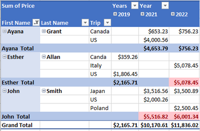
Thank you for your reply. I should have mentioned that I already tried doing that but it also shows if the grand total of the individual is greater than $5000 for all years instead of isolating for the subtotal of each year and checking that. Please see below. Thanks.

Dataset:

First Name Last NameTrip PriceYear

Esther	Allan	US	1806.45	2019-04-19
Esther	Allan	Canda	359.26	2019-07-20
Esther	Allan	Italy	5078.45	2022-05-04
John	Smith	US	2000.26	2021-02-02
John	Smith	Poland	2500.45	2022-05-05
John	Smith	Japan	3516.56	2021-05-07
John	Smith	Japan	3500.89	2022-07-04
Ayana	Grant	Canada	653.23	2021-03-05
Ayana	Grant	Canada	756.23	2022-04-09
Ayana	Grant	US	4000.56	2021-02-25
Jimmy	Lee	Canada	455.23	2019-04-19
Jimmy	Lee	Canada	454.56	2021-05-02
Jimmy	Lee	Canada	670.21	2021-07-02

[#4]

@zander140 Ah, I see. That would probably require a clever DAX measure. Not something I can help you with right now. Sorry!

[#5 · Accepted solution]

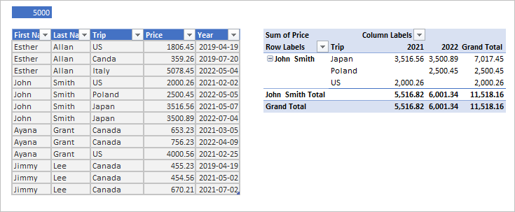
@zander140 

We may play with Power Query. For such model

first prepare the source table

let
    Source = Excel.CurrentWorkbook(){[Name="Table1"]}[Content],
    #"Changed Type" = Table.TransformColumnTypes(
        Source,
        {
            {"Year", type date},
            {"Price", Currency.Type},
            {"Trip", type text}
        }         ),
    #"Merged Columns" = Table.CombineColumns(
        #"Changed Type",
        {"First Name", "Last Name"},
        Combiner.CombineTextByDelimiter(" ", QuoteStyle.None),"Name"),
    #"Extracted Year" = Table.TransformColumns(
        #"Merged Columns",
        {{"Year", Date.Year, Int64.Type}})
in
    #"Extracted Year"

Next generate list of people who spent more than 5000 annually. We ignore years with no trips.

let
    Source = Table,
    Bar = Excel.CurrentWorkbook(){[Name="PriceBar"]}[Content]{0}[Column1],

    #"Grouped Rows" = Table.Group(
        Source,
        {"Name", "Year"},
        { {"Total", each List.Sum([Price]), type nullable number}}),
    #"Grouped Rows1" = Table.Group(
        #"Grouped Rows",
        {"Name"}, {{"Data", each List.Min( _[Total] ) > Bar }}),
    #"Filtered Rows" = Table.SelectRows(
        #"Grouped Rows1",
        each ([Data] = true)),
    #"Removed Other Columns" = Table.SelectColumns(
        #"Filtered Rows",{"Name"}),
    Name = #"Removed Other Columns"[Name]
in
    Name

Finally filter source table by these names and land query to the grid as PivotTable

let
    Source = Table,
    #"Filtered Rows" = Table.SelectRows(
        Source,
        each List.Contains(#"Names Filtered", [Name] ))
in
    #"Filtered Rows"

[#6]

Hi Sergei, Thank you very much. I thought Esther's data would show as well since her subtotal is greater than $5000 for 2022. I think what the program is doing is, it is removing Esther from the list since for 2019 her spent was only $2165.71. It would be great if any of the year had over $5000 as a subtotal it would show those (highlighted in red). Thanks. 

[#7]

@zander140 

Please see updated queries in attached file, result is

[#8]

@Sergei Baklan Thank you so much, Sergei. Can this method be used for a pre-existing Excel Table? Thank you. 

[#9]

@zander140 

In general yes, you need to adjust queries to actual data.

[#10]

@zander140 

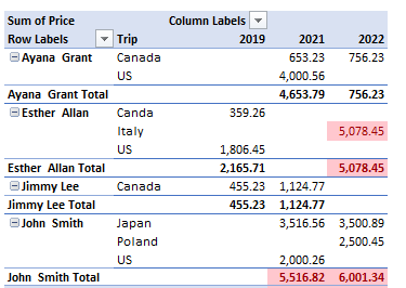
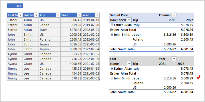
Another way could be with DAX measure only. Load you table and parameter to data model and use measure like

Cost :=
VAR bar =
    VALUES ( PriceBar[Bar] )
RETURN
    SUMX (
        Table1,
        IF (
            CALCULATE (
                SUM ( Table1[Price] ),
                ALLEXCEPT ( Table1, Table1[Name], Table1[Year (Year)] )
            ) > bar,
            Table1[Price],
            BLANK ()
        )
    )

Result is the same, see second PivotTable

[#11]

Thank you, Sergei. Thanks to you, I learned Power Query and applied it to my other project to do the same function. Power Query is amazing. I will look into DAX as well. Thank you.

[#12]

@zander140 , you are welcome, glad to help

[#13]

Hi Sergei, I thought everything was fine but when I put in new data and press refresh for the dataset I adapted your model for, I am getting the following error. Can you please help resolve this. Thanks.

[#14]

@zander140 

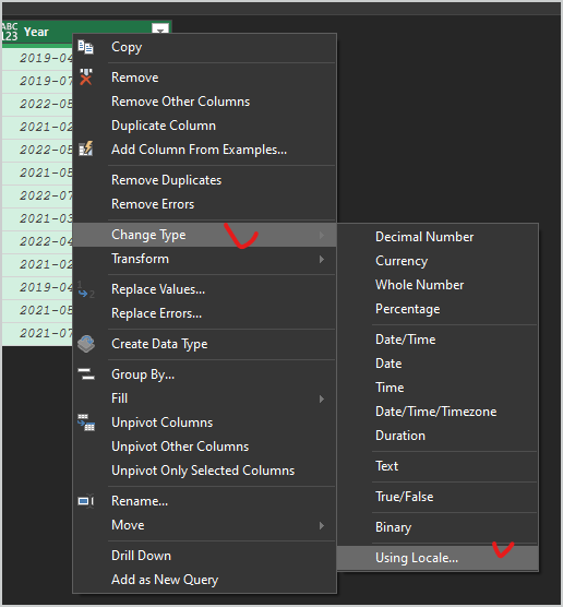
Perhaps you may share small sample file removing sensitive information? Your dates could be actually texts and/or format is not the same as default one for your Power Query locale. 

You may right click on the column on Source step, select column and from right click menu select

and here something like

Perhaps something else, hard to say without sample file.

[#15]

Hi Sergei, I sent you a direct message. Thank you.