Conditional formatting for entire row based on data in one cell

[AUSTXCHICK]

I need all cells in a row to highlight a certain color if the data in one cell contains a specific word. 

What I specifically want is for an entire row to turn grey if the status cell contains the word "SHIPPED." I know how to make that specific cell highlight the color I want, but not the entire row of the sheet.

Thank you for your help!

[#2]

@Ebony_T_0524 

Let's say you want to format rows from row 2 to row 100 that contain "sales" with possibly other text in column D.

Select rows 2 to 100.

The active cell in the selection should be in row 2, for example A2.

On the Home tab of the ribbon, click Conditional Formatting > New Rule...
Select 'Use a formula to determine which cells to format'.
Enter the formula

=ISNUMBER(SEARCH("sales", $D2))

Click Format...
Activate the Fill tab.
Select a highlight color.
Click OK, then click OK again.

[#3]

Worked perfectly. I only wanted to do certain columns in the row so I just switched the 'Applies to' to the columns I wanted.

Thanks Again

[#4]

Sorry to pile on with new question, but you all have such great responses! I'm using =LEFT(FILTER(range,criteria,"")10) to list only the first 10 characters from a filtered list of employees. I then want to conditionally format $B1:$J800 when the results of $C1 ="Text". If I use CF when text contains "Text", it will successfully highlight the cells containing "Text", but won't highlight the entire row, even if applies to $B1:$J800. If I use a formula to CF, it's never true because the cell doesn't ="Text", it equals the Filter formula. Any advice?

[#5]

@Renee Bugbee 

Select B1:J800. The active cell in the selection should be in row 1.

On the Home tab of the ribbon, click Conditional Formatting > New Rule...
Select 'Use a formula to determine which cells to format'.
Enter the formula

=ISNUMBER(SEARCH("Text",$C1))

Click Format...
Activate the Fill tab.
Select a highlight color.
Click OK, then click OK again.

[#6]

Super

[#7]

You're Awesome Hans!!! Works like a charm.
Thanks :)

[#8]

Regarding your reply/solution at 1348 hrs on 29 Aug, 2019, here, ::

This didn't work. I wanted to highlight b1:e1 when there is some specific text in a1. I've typed this conditional formula: =A1="some_text" and applied it to this: =$B$1:$E$1000. But when there is desired value in a1, only b1 is highlighted. I've tried many tries. Thanks again.

[#9]

@BathindaHelper 

Change the formula to

=$A1="some text"

The $ before the column letter A fixates the column, so that B1, C1, D1 and E1 all look at A1.

[#10]

it also worked with me, thank you

[#11]

@Sergei Baklan 

Hi Sergei, 

I am drawing blanks on a current issue I am having with the excel formatting (see snippet below). The table on the left side has over 4500 rows of hazardous material detail. I utilized a XLOOKUP formula for single row of data to automatically fill in the respective row on the large table by UN number. Is there a way to have this row automatically appear at the top so you don't have to scroll down. I highlighted the PSN, but would still have the row get filtered to the top. I hope I got the message across. Thank you! 

[#12]

@AUSTXCHICK 

Take a look at this 5 minute video instead of searching this page for half an hour :

https://youtu.be/XHT4paRaY4g                 Excel Conditional Formatting with Formula | How to Get it RIGHT Every Time

[#13]

@Sergei Baklan 

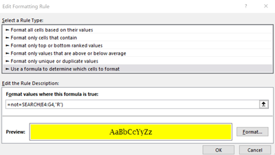
I need to be able to highlight A4 if E4:Q4 does not contain "R". I know how to do it for finding a value but not for not finding it. I have tried putting NOT in front of my formula but did not work.

[#14]

@MEdwards26 

Try

=COUNTIF(E4:Q4,"*R*")=0

or

=ISERROR(SEARCH("R",E4:Q4))

[#15]

Thank you very much. Particularly the last sentence of your answer that explained the reason as well. Thanks again. You people are really great.

[#16]

@AUSTXCHICK   thank you so much.  saved me a lot of aggro!

[#17]

lifesaver! Thanks a lot!

[#18]

so I am using version 16.66.1 and trying to do the same. So in column A (for say 100 rows) I want to highlight using the following format. If i put a 1 I want the row to be green. 2=yellow 3=white (no fill) or 4 is red. I am struggling to figure that out.

[#19]

Hello,

This a great learning thread.
I have a similar problem to solve. I have ColumnA of char data (ABC for example). I have another ColumnB of unique char data as reference. I want to highlight each row that contains a match with anyone one of the ColumnB reference values. I assume ColumnB needs to go on a separate tab?
Thank you!

[#20]

Hi Sergei! I used this to highlight the entire row if the columns from B to CP contain the specific texts I'm looking for. I also wanted to use the "AND" function as I'm looking for more than 1 text. But this didn't work for me. Is there another formula for this? Thanks!

[#21]

@dionne103 

For such range

if you'd like to highlight rows with BOTH abc and xyz conditional formatting rule formula could be

=SUMPRODUCT(  ($B2:$H2="abc") + ($B2:$H2="xyz") ) >= 2

, as