Conditional formatting for entire row based on data in one cell

[AUSTXCHICK]

I need all cells in a row to highlight a certain color if the data in one cell contains a specific word. 

What I specifically want is for an entire row to turn grey if the status cell contains the word "SHIPPED." I know how to make that specific cell highlight the color I want, but not the entire row of the sheet.

Thank you for your help!

[#2]

Here is a graphical example. Any cell in the data column that matches any one of the unique reference cells I want to highlight that row. Assume the Reference column needs to go on a separate tab?

[#3]

I am ecstatic. This is a game changer for me. Thank you!

[#4]

@Yury Tokarev 

Thanks this is great, is it possible to make it so it only changes the color of the row to a specific column rather than the entire row?

[#5]

@Yury Tokarev 

Good morning, 

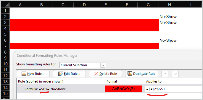
Appreciate the guidance you provided on this thread. for some reason, I inputted the instructions and for some reason when I select "No-show" from the drop down on Column " F" the red goes down a row. So it is not highlighting the row that the drop down in in. Please advise and thank you Yury. 

[#6]

@antmac 

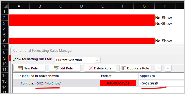
Most probably references in formula and in Apply To range are not in sync. For example

we use in formula reference with first row and apply to the range which starts from the second row. If to change on row 2 in formula, it works

[#7]

@Yury Tokarev 

I believe I have followed your instructions correctly, but the desired result only works in the first row.

The desired result is that any row from 5 to 500 that contains a qty other than zero in column F be highlighted.

Thank you in advance for your help.