Autofill Data

[sirk78]

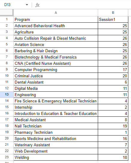
I am trying to speed up a process to autofill some data.  I am looking to find a formula that will check to see if B2 is less than 27, if it is return the value of A2, if not go to B3 to see if it is less than 27, if it is return A3, if not go to B4, and so on to the end of the list.  Any help would be appreciated.

[#2]

@sirk78 

If I read this correctly, you want the first program that's less than 27:

=INDEX(FILTER(program,session<27),1)

If you want all programs less than 27 then it's:

=FILTER(program,session<27)

[#3]

I gave that a try and it does return the correct values but I think I need to clarify what the outcome is. Currently, I am manually creating a list of participants in each program limited to 26 people. I have a list of names and I need to assign them to a program until it reaches its max, once the max is reached I move to the next program until it is filled, and so on until all programs have 26 or fewer participants. I do this currently by copying and pasting the name of the program next to a cell with a participant's name and the number under Session1 is updated automatically to reflect the new count. I am looking for a formula that will do this for me so that I can put a formula in the cell next to the name and have it automatically look at the list of programs and number of people assigned and if it is less than 27 it will add the program name, if not it will go to the next program on the list and the see if it has 27 or less.

I initially thought that a =IF or =IFS statement would work but I am missing something. I was thinking of something like this =IF(B2<27, A2,(if not go to B3 and if <27 return A3, if not go to B4 and so on down the list).

[#4]

It sounds do-able. It may need some recursion. Do you happen to have an example of the data arrangement with the participant names and programs?

[#5]

@Patrick2788 

Here is a modified version of the data. Some participants chose which program they wanted to attend but there are a lot that didn't which is why I have to fill in a program name.  This can be random. As mentioned I can do this manually but it would save time if I could add a formula on row E327 to do as i have described previously and then drag it down to the end of the participant name list so that everyone is in a program but less than 27 in each program. 

[#6 · Accepted solution]

@sirk78 

Thank you for the workbook.

Here's the formula. I treated this an 'unpacking' of the data. It's a bit longer because I had to avoid a circular reference with the totals in H.

=LET(
    counter, SEQUENCE(240),
    taken, COUNTIF(ProgramsBooked, program),
    available, 27 - taken,
    UnPack, LAMBDA(a, v, LET(resize, XLOOKUP(v, program, available, ""), VSTACK(a, EXPAND(v, resize, , v)))),
    Sessions_Available, DROP(REDUCE("", program, UnPack), 1),
    INDEX(Sessions_Available, counter)
)

. 

[#7]

Awesome thank you, it seems it wasn't as straightforward as I had thought. I appreciate the time you put into this!

[#8]

You're welcome! Glad I could help.