RAG status help

[robgill205]

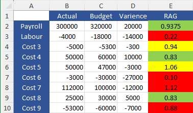
Hi, I've attached an example to help understanding.

I have applied conditional formatting to visualise a RAG status. The payroll status is working fine, as long as the figure is below 1.05 it will be green. Between 1.05-1.1 will be yellow, as it falls between the 5-10% overbudget range. Then red for over 10%.

The problem I have is I need to apply another rule that is applied when it sees that the budget figure is negative. If the budget figure is negative, then i want it to follow the rule set out below named Labour RAG. I need these two rules to be applied to an entire column and I don't know if it can work. Thank you in advance

[#2]

@robgill205 

Could you provide more examples, with the desired color manually indicated in a separate column?

[#3]

@Hans Vogelaar 

Sure, I hope this makes more sense. The current RAG status for the negative budget makes sense. It's saying the actual figure was not as negative as budgeted, therefore it is good. However I need it to ignore this logic and apply a separate rule.

[#4]

Row 4 should be yellow, sorry

[#5 · Accepted solution]

@robgill205 

You cannot do that with a rule of type icon sets. It's possible with two rules of type 'Use a formula to determine which cells to format'.

See the attached version. The cells have green as default fill color; the rules apply yellow or red depending on a formula that refers to columns C and E.

[#6]

Yeah I can use this format, thanks. Can you tell me how you got the cells as green for default?

[#7]

I should have asked this along with the other question, but is it also possible to hide the figures in the RAG too? So it only displays the fill colour. Thanks

[#8]

@robgill205 

Sure. I simply selected E2:E10 (or further down if required) and selected green as fill color.

In the attached version, the conditional formatting rules look at B2/C2 instead of at E2.

That allows us to clear the formulas from E2:E10.

[#9]

Thanks Hans.