How to apply separate conditional formatting rules for different Pivot Table Row Label sections

[wyse3]

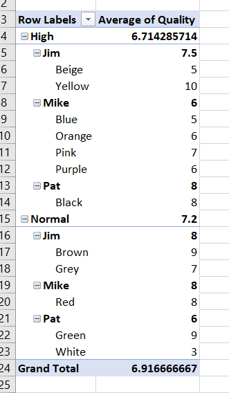
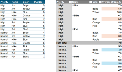
I have a pivot table that has two sections, a High Priority and Normal Priority section that needs different sets of conditional formatting rules, due to the High Priority section having higher standards etc. Is there a way to do this? So far I have only been able to apply rules to every row, not distinguishing between High and Normal priority. The attached table is a sample of how the table is structured. For example, I need to have one rule that fills red if the High Priority groups are under 7, and a rule that fills red if the Normal Priority groups are under 6.

[#2]

Hi @wyse3 

There's obviously something to do if you Show in Tabular Form + Repeat item labels for the Priority field;

Cond. Format rules that apply to All cells showing 'Average of Quality' values, with the above setup:

// High priority:
=AND($G3 = "high", $I3 <> "", $J3 < 7)

// Normal priority:
=AND($G3 = "normal", $I3 <> "", $J3 < 6)

the 2nd condition ($I3 <> "") in the above ANDs avoid highlighting numbers on the sub-total rows

[#3]

@wyse3 

On reflection when Excel 2021 or 365 is in use, that's doable w/o Repeating item labels in [Priority]

PS: In the event where the previous post solves the problem there's a Mark as response link at the bottom. Clicking it helps people who Search

[#4]

Hello,

I can't seem to get this to work without Repeating item labels. I am on 365. Is there anything different that needs to be done?

[#5]

Hi @wyse3 

I can't seem to get this to work without Repeating item labels

This means the initial proposed solution works but you didn't say so nor Mark as response... and now that you know it's doable without Repeating item labels with 2021 or 365 we hear from you. Not quite sure I understand

A suggestion in the meantime: take a look at the PS in my previous post