How can I sort values and color of data from highest to lowest.

[littlevillage]

Hi,

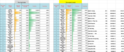
I want to sort values and color of data from highest to lowest.

I am trying to write the formula: 

=INDEX(SORT(FILTER(B3:F19,C3:C19>=LARGE(C3:C19,17),""),2,-1),SEQUENCE(17),{1,2,4,5})

It shows just only sorted values , the color is not

I have added an image and the link of the samplefile that shown the expect result

Hope for your help

Thank you

https://docs.google.com/spreadsheets/d/1WalOqGZk_5UFgJAow3n-MyE7Ggb2iPA7/edit?usp=sharing&ouid=11231... 

[#2 · Accepted solution]

I didn't/couldn't open the sheet in google docs but those bars sure look like conditional formatting and therefor will not appear on the new columns unless you add a new conditional formatting rule. Highlight one of the output columns go into conditional formatting and add a rule for color based on value and use data bars as the type or select the existing conditional formatting for column B and 'duplicate rule' and then change the 'applied to' range to the new range.

[#3]

@mtarler 

https://docs.google.com/spreadsheets/d/1acE_rzImeh0cR6Qi0CEeIC6NW4WOFhg-/edit?usp=sharing&ouid=11231... 

Have a look back please

[#4]

@littlevillage 

It is exactly what @mtarler wrote: the SORT formula only returns the sorted values. There is no way to make the formula also copy the conditional formatting of the source range.

You can use the format painter to copy the conditional formatting:

• Select C3:C19.
• Click the Format Painter button on the Home tab of the ribbon.
• Select N3 (or N3:N19).
• Select E3:E19.
• Click the Format Painter button on the Home tab of the ribbon.
• Select P3 (or P3:P19).

[#5]

@mtarler 

Thank for your help

It works correctly