Find and Replace Multiple Data Points (Or aDifferent Solution?)

[TimMarston]

Hi

I am using Microsoft Excel for Mac and am stumped with a problem.

I have a sheet with one column that has 340,000 rows of data.

I have a list of 350 names that I want to search the first column for.

But these names are only a part of the data in the column.

For example, if this was a row in the column:

https://techcommunity.microsoft.com/t5/forums/postpage/board-id/ExcelGeneral 

My list would only contain this:

techcommunity.microsoft.com

I am trying to delete any row in the column containing a name from the list of 350 names.

If I could highlight or ID the rows somehow, that could be workable as well, but deletion would be ideal.

Apart from doing this manually with find and replace, I have no idea how to do it.

My Excel skills are very limited.

I do no know if what I am asking is hard or easy, but it feels hard to me!

Any help would be much appreciated.

Thanks

Tim

[#2]

@TimMarston 

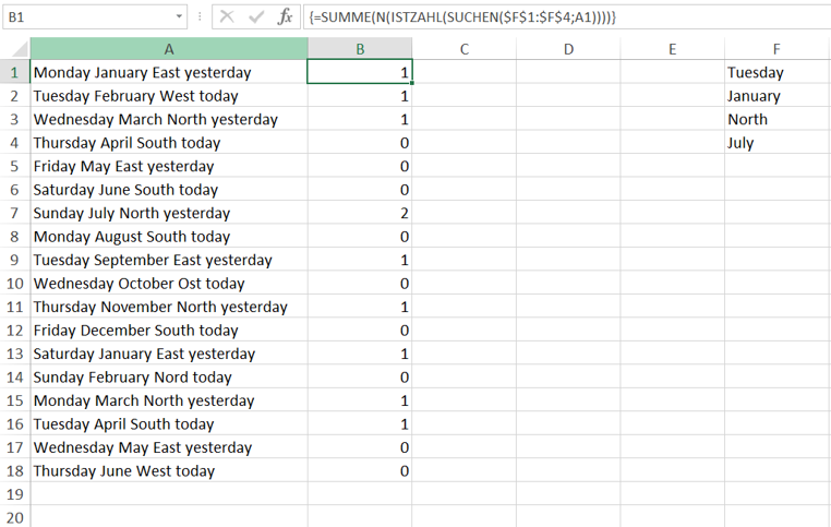
=SUM(N(ISNUMBER(SEARCH($F$1:$F$4,A1))))

You can apply this formula in the small example. Enter the formula with ctrl+shift+enter if you don't work with Office 365 or Excel for the web or Excel 2021.

The range of the formula can be changed according to your requirement e.g. 

=SUM(N(ISNUMBER(SEARCH($F$1:$F$350,A1))))

After applying the formula you can filter columns A and B and delete all rows where column B is greater 0. Then you can remove the filter. The remaining rows don't contain a name from the list of 350 names.

[#3]

@TimMarston

Select the list with the 350 names.

Click in the address box on the left hand side of the formula bar.

Type a name such as List then press Enter.

Let's say your data are in A2 and down.

In an empty column (insert one if necessary), enter the following formula in the cell in row 2:

=OR(ISNUMBER(SEARCH(List, A2)))

Fill down to the last used row. If the data column doesn't contain blank cells, the easiest way to do that is to double-click the fill handle in the lower right corner of the cell with the formula.

You'll now have a column with TRUE/FALSE values - TRUE if the cell in column A contains at least one of the names from the list, FALSE otherwise.

Filter the column to display only the TRUE values.

Select all visible rows from row 2 down, then delete them.

Finally, turn the filter off.

[#4]

@Hans Vogelaar  Thanks, Hans. I appreciate the help.

When you say, "Select the list with the 350 names." Currently, that list is in a txt file.

Should it be added to the sheet I am working on? In the same tab?

When you say, "Click in the address box on the left-hand side of the formula bar."

I'm not sure what you mean.

I think I know what the formula bar is, but I can't find the address box.

This is what I am currently looking at:

Where do I find theaddress box?

[#5]

@TimMarston 

Copy the list of names into a range on a worksheet - it can be the sheet with the data, or another sheet in the same workbook. That doesn't matter.

[#6]

Thanks Hans.

I got it working somewhat, but it seems to throw up many false positives.

If you look at this image (sorry for the content; I'm trying to remove spam links from a client's site).

You can see the first two rows worked as they should have.

When I scroll down the sheet, a lot of values say TRUE when I dont think they should.

You can see the example in the image:

I have manually searched column E and A13 should not be listed as true.

I am not sure what I am doing wrong?

[#7]

@TimMarston 

Are you sure that datissamaneh.ir (or part of it, for example amaneh.ir) is not in your list of spam domains?