- Home
- Microsoft 365
- Excel
- Need help to resolve Excel Formula using Let,Take,index,Sort,Unique,HSTACK,MMULT,TOROW,MONTH.
Need help to resolve Excel Formula using Let,Take,index,Sort,Unique,HSTACK,MMULT,TOROW,MONTH.
- Subscribe to RSS Feed
- Mark Discussion as New
- Mark Discussion as Read
- Pin this Discussion for Current User
- Bookmark
- Subscribe
- Printer Friendly Page
- Mark as New
- Bookmark
- Subscribe
- Mute
- Subscribe to RSS Feed
- Permalink
- Report Inappropriate Content
Aug 18 2023 01:31 PM
I am trying to add 5 additional columns to the function but can get only a $value:
Function :
=LET(r,B1:G8,m,6,a,TAKE(r,,1),b,INDEX(r,,2),c,INDEX(r,,3),d,INDEX(r,,4),e,INDEX(r,,5),f,INDEX(r,,6),g,INDEX(r,7),u,SORT(UNIQUE(a)),HSTACK(u,MMULT(--(TOROW(a)=u),(MONTH(b)=m)*c)))
Data
A B C D E F G
Chequing 06962-5001375 2023-08-01 " " INSURANCE IND ALL AC-EST -203.64
Chequing 06962-5001375 2023-08-01 " " INSURANCE THE PERSONAL -269.88
Chequing 06962-5001375 2023-08-02 " " OD HANDLING FEE 1 @ $ 5.00 -5
Chequing 06962-5001375 2023-08-09 " " Transfer WWW TRANSFER - 0982 1000.00
Chequing 06962-5001375 2023-08-09 " " Payment WWW PAYMENT - 5925 MILTON - TAXE -50
Chequing 06962-5001375 2023-08-09 " " Payment WWW PAYMENT - 2317 RELIANCE -55
Chequing 06962-5001375 2023-08-09 " " Payment WWW PAYMENT - 8635 MILTON HYDRO -145.52
Chequing 06962-5001367 2023-04-18 OD INTEREST -3.7
Result #VALUE
If I use a subscript of the data i.e. 3 col The function is of:
Function:
=LET(r,A1:G8,m,6,a,TAKE(r,,1),b,INDEX(r,,2),c,INDEX(r,,3),u,SORT(UNIQUE(a)),HSTACK(u,MMULT(--(TOROW(a)=u),(MONTH(b)=m)*c)))
Data:
06962-5001375 2013-06-10 2.00
06962-5001375 2013-06-10 3.00
06962-5001375 2013-05-13 4.00
06962-5001375 2013-05-14 5.00
06962-5001375 2013-06-15 6.00
06962-5001380 2013-06-17 7.00
03092-5224710 2013-06-17 8.00
03092-5224710 2013-06-18 9.00
Result:
06962-50011121 3
06962-50011122 3
06962-50011123 6
Thanks tp P. b. at stack overflow for the original suggestion.
How do I add in the extra columns?
I would appreciate any help that you can provide me
Thanking you in advance.
- Labels:
-
Excel
- Mark as New
- Bookmark
- Subscribe
- Mute
- Subscribe to RSS Feed
- Permalink
- Report Inappropriate Content
Aug 18 2023 02:02 PM
In general your formula
=LET(
    r, B1:G8,
    m, 8,
    a, TAKE(r, , 1),
    b, INDEX(r, , 2),
    c, INDEX(r, , 3),
    d, INDEX(r, , 4),
    e, INDEX(r, , 5),
    f, INDEX(r, , 6),
    g, INDEX(r, 7),
    u, SORT(UNIQUE(a)),
    HSTACK(u, MMULT(--(TOROW(a) = u), (MONTH(b) = m) * c))
)
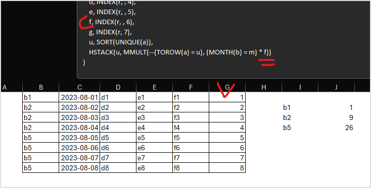
works, e.g.
but I was not able to paste your sample into the grid and didn't catch what exactly you try to do.
- Mark as New
- Bookmark
- Subscribe
- Mute
- Subscribe to RSS Feed
- Permalink
- Report Inappropriate Content
Aug 18 2023 02:07 PM
- Mark as New
- Bookmark
- Subscribe
- Mute
- Subscribe to RSS Feed
- Permalink
- Report Inappropriate Content
Aug 19 2023 06:42 AM
B E F G
06962-5001375 INSURANCE IND ALL AC-EST -203.64
06962-5001375 INSURANCE THE PERSONAL -469.88
06962-5001375 OD HANDLING FEE 1 @ $ 5.00 -5
06962-5001375 Transfer WWW TRANSFER - 0982 1000.00
DATA
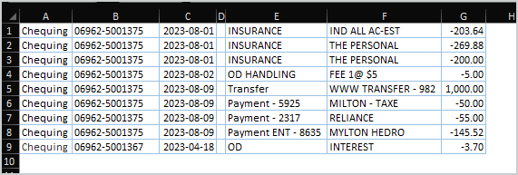
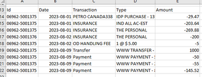
A B C D E F G
1 Chequing 06962-5001375 2023-08-01 " " INSURANCE IND ALL AC-EST -203.64
2 Chequing 06962-5001375 2023-08-01 " " INSURANCE THE PERSONAL -269.88
3 Chequing 06962-5001375 2023-08-01 " " INSURANCE THE PERSONAL -200.00
4 Chequing 06962-5001375 2023-08-02 " " OD HANDLING FEE 1 @ $ 5.00 -5
5 Chequing 06962-5001375 2023-08-09 " " Transfer WWW TRANSFER - 0982 1000.00
6 Chequing 06962-5001375 2023-08-09 " " Payment - 5925 MILTON - TAXE -50
7 Chequing 06962-5001375 2023-08-09 " " Payment - 2317 RELIANCE -55
8 Chequing 06962-5001375 2023-08-09 " " Payment ENT - 8635 MILTON HYDRO -145.52
Chequing 06962-5001367 2023-04-18 OD INTEREST -3.7
i removed www for readability only.
I hope I have got it right this time. I have been trying to get this right for at least two weeks and it is driving me crazy.
- Mark as New
- Bookmark
- Subscribe
- Mute
- Subscribe to RSS Feed
- Permalink
- Report Inappropriate Content
Aug 19 2023 08:37 AM
Sorry, I still can't understand how the source data is structured. Is that as
? If so what is the logic behind generating these 4 output records, why these ones not another? Or your output doesn't cover entire input?
- Mark as New
- Bookmark
- Subscribe
- Mute
- Subscribe to RSS Feed
- Permalink
- Report Inappropriate Content
Aug 19 2023 05:37 PM - edited Aug 20 2023 12:05 PM
This is the entire Source data, I need to have the data structured so that I can have B, F, G By G
i.e.
Output
06962-5001375 INSURANCE IND ALL AC-EST -203.64
06962-5001376 INSURANCE THE PERSONAL -469.88
06962-5001377 OD HANDLING FEE 1 @ $5 5
..
..
..
..
06962-5001367 OD HANDLING INTEREST 3.7
Sorry for the confusion my snip & sketch does not want to paste the snip. However, the above is what my output should look like.
Thanks for the support and patience in helping me resolve this issue.
- Mark as New
- Bookmark
- Subscribe
- Mute
- Subscribe to RSS Feed
- Permalink
- Report Inappropriate Content
Aug 20 2023 12:32 PM
Chequing 06962-5001375 2023-04-18 C-IDP PURCHASE-3770 NOFRILLS JOHN'S -33.8
Chequing 06962-5001375 2023-04-18 OD INTEREST -0.92
Chequing 06962-5001375 2023-04-19 C-IDP PURCHASE-2812 LUNCHBOX CAFE -2.95
Chequing 06962-5001375 2023-04-19 C-IDP PURCHASE-9840 NOFRILLS JOHN'S -4.58
Chequing 06962-5001375 2023-04-19 C-IDP PURCHASE-9364 FOOD BASICS 88 -44.36
Sergei Sorry for all the confusion, I am trying to have the columns B, C ,E, F, G Displayed by month, by E, by F, by G.
the formula does this but with the by month and by B, E, F, G only if I change the UNIQUE and TOROW statements to the applicable TAKE variable. i.e
=LET(r,B1:G6,
m,4,
x,E1:E6,
a,TAKE(r,,1),
b,INDEX(r,,2),
c,INDEX(r,,3),
d,INDEX(r,,4),
e,INDEX(r,,5),
f,INDEX(r,,6),
v,VLOOKUP(x,x,1,FALSE),
u,SORT(UNIQUE(v)),
HSTACK(u,MMULT(--(TOROW(v)=u),(MONTH(b)=m)*f)))
OUTPUT
C-IDP PURCHASE-2812 -2.95
C-IDP PURCHASE-3770 -33.8
C-IDP PURCHASE-9364 -44.36
C-IDP PURCHASE-9840 -4.58
OD INTEREST -0.92
PETRO-CANADA -29.42
if I change the UNIQUE to "a" and TOROW to "a" my output changes to:
06962-5001375 -116.03
is this the right way to look at the data or can you suggest something else. I am open for any suggestions as I have spent far to many hours on this subject.
- Mark as New
- Bookmark
- Subscribe
- Mute
- Subscribe to RSS Feed
- Permalink
- Report Inappropriate Content
Aug 21 2023 06:25 AM
To add screenshot here, copy it into clipboard, here click on Insert Picture button
after that click by mouse at any place in grey area
Ctrl+V, picture shall be loaded from the clipboard, when it's ready click Done at bottom right.
Back to the sample, I added headers for better understanding, in general you may ignore them.
I guess we need to sum amount for identical Id, Date, Transaction and Type. That could be done by
=LET(
    range, $B$2:$G$10,
    Id, CHOOSECOLS(range, 1),
    date, CHOOSECOLS(range, 2),
    transaction, CHOOSECOLS(range, 4),
    type, CHOOSECOLS(range, 5),
    amount, CHOOSECOLS(range, 6),
    groupIndexes, {1,2,4,5},
    group, UNIQUE( CHOOSECOLS(range, groupIndexes ) ),
    VSTACK({"Id","Date","Transaction","Type","Amount"},
    HSTACK(
        group,
        BYROW( group,
            LAMBDA(v, SUM(
                FILTER(amount,
                    (Id = INDEX(v,1,1) )*
                    (date = INDEX(v,1,2) )*
                    (transaction = INDEX(v,1,3) )*
                    (type = INDEX(v,1,4) )
                )
            ) )
        )
    ) )
)
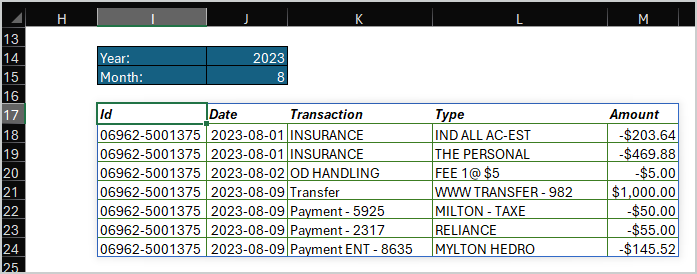
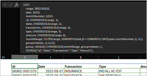
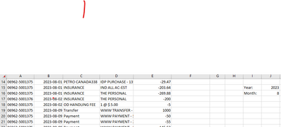
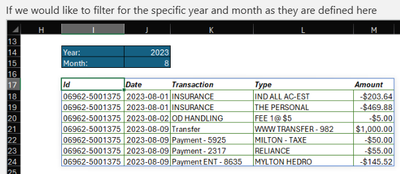
If we would like to filter for the specific year and month as they are defined here
slightly modified formula will be
=LET(
    range, $B$2:$G$10,
    year, $J$14,
    monthNumber, $J$15,
    Id, CHOOSECOLS(range, 1),
    date, CHOOSECOLS(range, 2),
    transaction, CHOOSECOLS(range, 4),
    type, CHOOSECOLS(range, 5),
    amount, CHOOSECOLS(range, 6),
    monthRange, FILTER(range, EOMONTH(date,0) = EOMONTH( DATE(year,monthNumber,1), 0 )),
    groupIndexes, {1,2,4,5},
    group, UNIQUE( CHOOSECOLS(monthRange, groupIndexes ) ),
    VSTACK({"Id","Date","Transaction","Type","Amount"},
    HSTACK(
        group,
        BYROW( group,
            LAMBDA(v, SUM(
                FILTER(amount,
                    (Id = INDEX(v,1,1) )*
                    (date = INDEX(v,1,2) )*
                    (transaction = INDEX(v,1,3) )*
                    (type = INDEX(v,1,4) )
                )
            ) )
        )
    ) )
)
Your initial formula sum amounts for the unique Id (only one column) in a given month. It's can't be adjusted directly for the few unique columns.
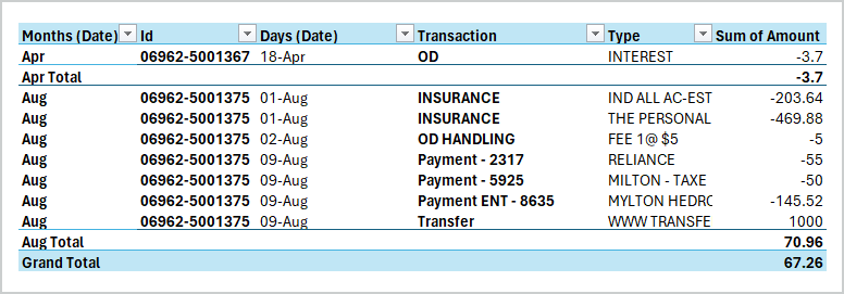
Another way is to create PivotTable, something like
Please check in attached file if that close to what you'd like to receive.
- Mark as New
- Bookmark
- Subscribe
- Mute
- Subscribe to RSS Feed
- Permalink
- Report Inappropriate Content
Aug 21 2023 06:12 PM
Once again thank you for your kind help. It has been a long three weeks since I started this project.
- Mark as New
- Bookmark
- Subscribe
- Mute
- Subscribe to RSS Feed
- Permalink
- Report Inappropriate Content
Aug 22 2023 01:13 AM
@Norman_McIlwaine , thank you for the feedback.
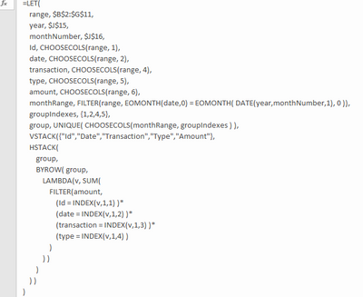
Above is just formula which you may edit directly in formula bar. If you check the file from previous post it's here
but practically not visible if you don't expand formula bar. For that click on any empty place within it and Ctrl+Shift+U. Or drag bottom border down.
Editing here use Alt+Enter to insert new line.
In addition you may install Excel Labs add-in from the Store
within it it'll be Advanced Formula Environment to work with formulae and not only.
- Mark as New
- Bookmark
- Subscribe
- Mute
- Subscribe to RSS Feed
- Permalink
- Report Inappropriate Content
Aug 22 2023 11:01 AM
Thank you Sergei for the valuable information, I very much appreciate it. I used the formula on the data unfortunately the amount was not summed i.e. The Personal in rows 4 and 5. I tried to review the formula only changing the year and date variables to correspond with the input in col J. The rest I could follow in a basic form however , I could not see where the calculation was taking place to give the sum amount. is it the LAMBDA I see that is were you do all the sum. However, I cannot figure it out at this time.
Thanks Sergei for all the help given.
- Mark as New
- Bookmark
- Subscribe
- Mute
- Subscribe to RSS Feed
- Permalink
- Report Inappropriate Content
Aug 22 2023 11:15 AM
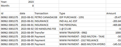
Formula works, correctly, perhaps I misunderstood the logic. It sums the values if only each of the value in these 4 columns are the same:
For them only INSURANCE in column C is the same value, thus they are not summarised. Which exactly fields shall be the same to summarize amounts?
- Mark as New
- Bookmark
- Subscribe
- Mute
- Subscribe to RSS Feed
- Permalink
- Report Inappropriate Content
Aug 22 2023 12:05 PM
Sorry for the misunderstanding, in a previous image you had it right.
In a previous capture you got it just right the C and D where the same so it added the amount.
- Mark as New
- Bookmark
- Subscribe
- Mute
- Subscribe to RSS Feed
- Permalink
- Report Inappropriate Content
Aug 25 2023 07:31 AM
@Norman_McIlwaine Sergei, If I change the date(day) to a 1 The function works great, Is there anyway we can add in a piece of code to perform a unique when the function is finished I have tried several ways to include this into the function but have failed every time. I even wrote a separate piece of code which I got from the You Tube and adapted it to test my data prior to inserting however I get the same results frustration.
Can you please help me Sergei?
- Mark as New
- Bookmark
- Subscribe
- Mute
- Subscribe to RSS Feed
- Permalink
- Report Inappropriate Content
Aug 25 2023 07:43 AM
Could you please clarify what shall be unique, or, perhaps, you could manually generate desired result? I see now rows which have the same values in all columns, thus formula returns an array as it is.
- Mark as New
- Bookmark
- Subscribe
- Mute
- Subscribe to RSS Feed
- Permalink
- Report Inappropriate Content
Aug 25 2023 11:27 AM
Original Data
The above formula will only work if the fields C,D,F are of the same value
Changed Original date to 2023-08-01 from 2023-08-02
The above formula works great,
If the date in column D5 are the same as column D4 2023-08-01
the Type field is then UNIQUE and the amount is summed as well.
I need the Transaction and Type fields to be unique. In other words I am trying to not have all three fields the same just two.
Thanks for all the help you have provided to me.
- Mark as New
- Bookmark
- Subscribe
- Mute
- Subscribe to RSS Feed
- Permalink
- Report Inappropriate Content
Aug 25 2023 11:46 AM
Okay, thank you. If the dates in D4 and D5 are different, which date shall we show combining these two records, or we don't show dates at all in output?
- Mark as New
- Bookmark
- Subscribe
- Mute
- Subscribe to RSS Feed
- Permalink
- Report Inappropriate Content
Aug 25 2023 01:50 PM
I removed the dates and found the formula worked well except I could not select by month. I don't need the dates at all in the output since we should will be selecting by year month.
The end result is good.
How can I select the data by Year and Month?
- Mark as New
- Bookmark
- Subscribe
- Mute
- Subscribe to RSS Feed
- Permalink
- Report Inappropriate Content
Aug 26 2023 04:06 AM
To exclude dates what we shall do in formula is to remove/change related indexes
This part of the formula
monthRange, FILTER(range, EOMONTH(date,0) = EOMONTH( DATE(year,monthNumber,1), 0 )),is filtering source range for the selected month, we keep it unchanged
Finally entire formula is
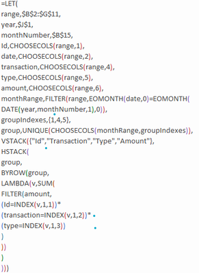
=LET(
    range, $B$2:$G$10,
    year, $J$14,
    monthNumber, $J$15,
    Id, CHOOSECOLS(range, 1),
    date, CHOOSECOLS(range, 2),
    transaction, CHOOSECOLS(range, 4),
    type, CHOOSECOLS(range, 5),
    amount, CHOOSECOLS(range, 6),
    monthRange, FILTER(range, EOMONTH(date,0) = EOMONTH( DATE(year,monthNumber,1), 0 )),
    groupIndexes, {1,4,5},
    group, UNIQUE( CHOOSECOLS(monthRange, groupIndexes ) ),
    VSTACK({"Id","Transaction","Type","Amount"},
    HSTACK(
        group,
        BYROW( group,
            LAMBDA(v, SUM(
                FILTER(amount,
                    (Id = INDEX(v,1,1) )*
                    (transaction = INDEX(v,1,2) )*
                    (type = INDEX(v,1,3) )
                )
            ) )
        )
    ) )
)
which returns
Please check in No Dates sheet attached.
Aug 26 2023 02:19 PM - last edited on Nov 13 2023 09:50 AM by
- Mark as New
- Bookmark
- Subscribe
- Mute
- Subscribe to RSS Feed
- Permalink
- Report Inappropriate Content
Aug 26 2023 02:19 PM - last edited on Nov 13 2023 09:50 AM by
I found this to be very good on the small amount of data. When I expanded the data over several months (8,4) I found the amount is summed over all months while the output from Id, Transaction, and Type are only selecting by the month requested.
Example PETRO
Accepted Solutions
- Mark as New
- Bookmark
- Subscribe
- Mute
- Subscribe to RSS Feed
- Permalink
- Report Inappropriate Content
Sep 07 2023 08:15 AM
SolutionThank you. Do I understand correctly that csv62719 is you source file. If to avoid Power Query we copy/paste data from it into the sheet in main file, here by formula create massaged range and based on it and month/year/monthid parameters create aggregated result. Workflow is correct?

