Coping Conditional Formatting to other cells and update the condition based on the copied to cells.

[Kingsnake]

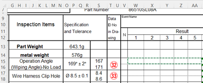
Example Cell Value - not between CELL 1 and CELL2. 

Then copy the same condition to other cells but apply not between CELL3 and CELL4.

When I copy I want the CELL S15 and CELL S16 to change to CELL S17 and CELL S18.

[#2 · Accepted solution]

@Kingsnake 

Let's say the rule as shown applies to a cell or cells in row 3.

Change the formulas in the rule to

=INDEX($S:$S, 2*(ROW(A3)-ROW(A$3))+15)

and

=INDEX($S:$S, 2*(ROW(A3)-ROW(A$3))+16)

[#3]

@Hans Vogelaar 

I have created a conditional formatting on cells W15, X15, Y15, Z15, and AA15 as shown below.

I want to copy this conditional format to cells W17, X17, Y17, Z17, and AA17 and have the evaluation cells for the condition change with the copy to be "not between" S17 and S18.

However when I try to copy and paste only the format to W17 ~ AA17, the evaluation cells do not change. They remain S15 and S16. I have also tried to highlight cells W15 ~ AA15 and use the format painter but that does not work either.

Maybe there is no way to do this in Excel.

I have set up a condition that if the any of the values in W15 ~ AA15 is not between the parameters in S15 and S16, then the value turns RED.

After setting this condition for the cells W15 ~ AA15, I then want to copy this condition to Cells W17 ~ AA17 but have the parameter values change to between S17 and S18.

Is this not possible? 

[#4]

@Kingsnake 

Change the formulas =$S$15 and =$S$16 to =$S15 and $S16, i.e. no $ before the row numbers 15 and 16.

Copy > Paste Formats should work then, and the Format Painter too

[#5]

To Mr. Hans,
Thank You!
That solution worked.
Thank you for your help!