How to assign numerical value to a list?

[SleepyTiger2013]

Hello,

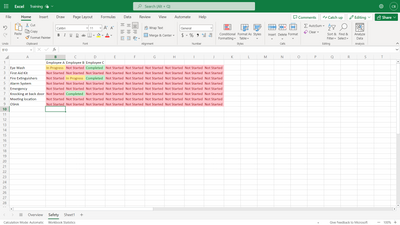
I am currently working on a new training program for my team and I am running into a little difficulty with formatting. I'd like to get this set so that the selected cell will "read" the cells above it in the column as a numerical value to calculate a percent complete. 

"Not Started" should be read as a 0 or 0%

"In Progress" should be read as a 1 or 50%

"Completed" should be read as a 2 or 100%

Ideally, then I'd like to have the selected cell tally each cell's value and give me a red, yellow, or green read-out based on how much they have completed. So for example: Column C could be read as 25% Completed, but overall, less than 50% so still RED. 

Any help or recommendations for this is appreciated. 

-Cathy

[#2 · Accepted solution]

@SleepyTiger2013 

In Excel for the web, you can use the following approach to assign numerical values to your list and calculate the percent complete:

1. Select the cell where you want to display the percent complete.
2. Go to the "Insert" tab in the Excel for the web toolbar and click on "Dropdown."
3. In the dropdown menu, select "Data Validation."
4. In the data validation settings, choose "List" as the validation criteria.
5. In the "Source" field, enter the following values: "Not Started,In Progress,Completed" (without quotes).
6. Click "OK" to apply the data validation to the selected cell.
7. Now, in a separate cell, you can use the following formula to calculate the percent complete based on the selected value:

=IF(A1="Not Started",0,IF(A1="In Progress",50,IF(A1="Completed",100,"")))

Replace A1 with the cell reference of the selected cell.

This formula checks the value in the selected cell and assigns the corresponding numerical value: 0 for "Not Started," 50 for "In Progress," and 100 for "Completed."

To get the overall progress color read-out, you can use conditional formatting based on the calculated percent complete. Select the range of cells you want to format, go to the "Home" tab, click on "Conditional Formatting," and choose "Color Scales" or "Icon Sets" to apply color formatting based on the percent complete.

Please note that Excel for the web may have limitations compared to the desktop version, so some advanced features may not be available.

[#3]

Thank you so much! This has worked wonderfully!