- Subscribe to RSS Feed
- Mark Discussion as New
- Mark Discussion as Read
- Pin this Discussion for Current User
- Bookmark
- Subscribe
- Printer Friendly Page
- Mark as New
- Bookmark
- Subscribe
- Mute
- Subscribe to RSS Feed
- Permalink
- Report Inappropriate Content
Feb 20 2024 03:11 AM
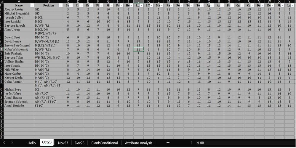
Below is the screenshot of my spreadsheet:-
I’m currently on the tab Oct23, this is the start data.
Next tabs is Nov23, Dec23 and so on.
What I’m wanting to do is add the new data to Nov23 tab and have the cell colour change based on the number difference to Oct23.
What I’m looking for is:-
Red cell if -2 & below
Light red if -1
No change if the same
Dark green if +1
Light green if +2 & above
The full spread sheet is:-
Coloumns = A to AQ
Rows = 2 to 99
How do I do this?
I know its conditional formatting, but how do I set this up?
- Labels:
-
Excel
-
Formulas and Functions
- Mark as New
- Bookmark
- Subscribe
- Mute
- Subscribe to RSS Feed
- Permalink
- Report Inappropriate Content
Feb 20 2024 03:28 AM
Will the names in column A be the same each month, in the same order? If so:
Select C2:AQ99 on the Nov23 sheet.
C2 should be the active cell in the selection.
On the home tab of the ribbon, click Conditional Formatting > New Rule...
Select 'Format only cells that contain'.
Leave the first drop down set to 'Cell Value'.
Select 'less than or equal to' from the second drop down.
In the box next to it, enter the formula
=Oct23!B2
Click Format...
Activate the Fill tab.
Select red as fill color.
Click OK, then click OK again.
Repeat these steps, but with 'equal to', =Oct23!B2-1 and light red.
Repeat them again, with 'equal to', =Oct23!B2+1 and dark green.
Finally, with 'greater than or equal to', =Oct23!B2+2 and light green.
- Mark as New
- Bookmark
- Subscribe
- Mute
- Subscribe to RSS Feed
- Permalink
- Report Inappropriate Content
Feb 20 2024 06:16 AM
But would the formulas be different if the list of names changed? It's a game so I'll be buying and selling players.
The spreadsheet is a stat tracker to see if my players are improving or declining.
- Mark as New
- Bookmark
- Subscribe
- Mute
- Subscribe to RSS Feed
- Permalink
- Report Inappropriate Content
Feb 20 2024 07:31 AM
If the names in column A change from month to month, the formulas in the rules become more complicated. In each of the rules, replace Oct23!B2 with
INDEX(Oct23!B:B, MATCH($A2, Oct23!$A:$A. 0))
or with
XLOOKUP($A2, Oct23!$A:$A, Oct23!B:B)
- Mark as New
- Bookmark
- Subscribe
- Mute
- Subscribe to RSS Feed
- Permalink
- Report Inappropriate Content
Feb 20 2024 07:40 AM
So I know which one is +1 (Dark green), +2 (Light Green), -1 (Light red), -2 (Red).
I'm totally new to excel & have learning difficulties, your first post was perfect for me and made total sense, I looked all over for help and your the first to explain the way I understand. Thank you
- Mark as New
- Bookmark
- Subscribe
- Mute
- Subscribe to RSS Feed
- Permalink
- Report Inappropriate Content
Feb 20 2024 07:50 AM
Here is my first reply, modified:
Will the names in column A be the same each month, in the same order? If so:
Select C2:AQ99 on the Nov23 sheet.
C2 should be the active cell in the selection.
On the home tab of the ribbon, click Conditional Formatting > New Rule...
Select 'Format only cells that contain'.
Leave the first drop down set to 'Cell Value'.
Select 'less than or equal to' from the second drop down.
In the box next to it, enter the formula
=XLOOKUP($A2, Oct23!$A:$A, Oct23!B:B)
Click Format...
Activate the Fill tab.
Select red as fill color.
Click OK, then click OK again.
Repeat these steps, but with 'equal to', =XLOOKUP($A2, Oct23!$A:$A, Oct23!B:B)-1 and light red.
Repeat them again, with 'equal to', =XLOOKUP($A2, Oct23!$A:$A, Oct23!B:B)+1 and dark green.
Finally, with 'greater than or equal to', =XLOOKUP($A2, Oct23!$A:$A, Oct23!B:B)+2 and light green.
- Mark as New
- Bookmark
- Subscribe
- Mute
- Subscribe to RSS Feed
- Permalink
- Report Inappropriate Content
Feb 20 2024 10:59 AM
What's the B:B at the end?
Guess I'll have to stick with the first way. Might try find someone to send the sheet to and ask if they can set it up and send it back. Would that work??
- Mark as New
- Bookmark
- Subscribe
- Mute
- Subscribe to RSS Feed
- Permalink
- Report Inappropriate Content
Feb 20 2024 11:47 AM
Could you attach a small sample workbook demonstrating the problem (without sensitive data), or if that is not possible, make it available through OneDrive, Google Drive, Dropbox or similar?
- Mark as New
- Bookmark
- Subscribe
- Mute
- Subscribe to RSS Feed
- Permalink
- Report Inappropriate Content
Feb 20 2024 12:07 PM
Xlookup - is what I'm struggling with, cannot seem to get that working.
https://drive.google.com/drive/folders/1v8loMjCktN7xcz4SQeFACL47WdBsCS9f?usp=sharing
- Mark as New
- Bookmark
- Subscribe
- Mute
- Subscribe to RSS Feed
- Permalink
- Report Inappropriate Content
Feb 20 2024 12:27 PM
Sorry - my mistake. The formulas should have used Oct23!C:C instead of Oct23!B:B.
See the attached version.
