Function Help

[AL789]

Hi all.
I'm hoping to get some help writing a function. I need something that can look up a project number in another tab and count associated data from other columns to bring into the new tab. I attached a sample file of what my data looks like and how I want the resulting formula to be displayed.

Any ideas?

[#2]

@AL789 

I think what you need, rather than a Function, is a different way of thinking of your data. See the attached. I've reconfigured your data into a different kind of table, and then used Excel's Pivot Table capability to summarize the data. I believe the summary gives you exactly the kind of accounting you need.

You'll notice that I used VLOOKUP to populate the final column in the new table. It might be just as useful to use a drop-down (under Data Validation) to give yourself a choice of consistent labels for that column, rather than a number and a VLOOKUP.

You may or may not want to put the NAME of your partners in, and I just put junk in there, but it serves as a field to produce the count. But the Pivot Table is an excellent and easy (once you master it) way to produce the kind of summary data you're seeking.

[#3]

Thank you for your response! This works to produce the data I require, though due to the way I must integrate the final results with my other program data, I would like to use a function instead. I'm hoping this is something that can be done with a function (or multiple functions)

[#4]

@AL789 

Start this formula in the Counts sheet, cell B2:

=SUM(IF(OFFSET(Data!$A$1,MATCH($A2,Data[[Project ]],0),1,1,7)=SUBSTITUTE(SUBSTITUTE(B$1,"Number of ","")," Partners",""),1,0))

Ctrl+shift+enter

Please read @mathetes 's suggestion. It's great advice unless you prefer to write complex array formulas.

[#5 · Accepted solution]

@AL789 

One more variant

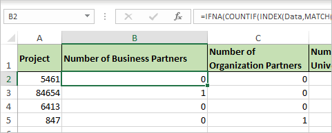
in B2

=IFNA(COUNTIF(INDEX(Data,MATCH($A2,Data[[Project ]:[Project ]],0),),SUBSTITUTE(SUBSTITUTE(B$1,"Number of ","")," Partners","")),0)

and drag it to the right and down

[#6]

@AL789 

And one more variant with Power Query

Generated script

let
    Source = Excel.CurrentWorkbook(){[Name="Data"]}[Content],
    UnpivotOtherColumns = Table.UnpivotOtherColumns(
        Source,
        {"Project "},
        "Attribute", "Value"
    ),
    FilterBlanks = Table.SelectRows(
        UnpivotOtherColumns,
        each ([Value] <> "NULL" and [Value] <> "Off")
    ),
    ModifyNames = Table.ReplaceValue(
        FilterBlanks,
        each [Value],
        each "Number of " & [Value] & " Projects",
        Replacer.ReplaceValue,{"Value"}
    ),
    RemoveProjectType = Table.RemoveColumns(
        ModifyNames,
        {"Attribute"}
    ),
    AddIndex = Table.AddIndexColumn(
        RemoveProjectType,
        "Index", 1, 1
    ),
    PivotProjects = Table.Pivot(
        AddIndex,
        List.Distinct(AddIndex[Value]),
        "Value", "Index", List.Count
    )
in
    PivotProjects

[#7]

I need someone to give the steps to merge a data base in excel to mailing labels in word.

[#8]

@Betty58 

That's a separate question, please start new conversation here https://techcommunity.microsoft.com/t5/excel/bd-p/ExcelGeneral