Duplicate values with partial matches

[subbucat]

Hello Gurus,

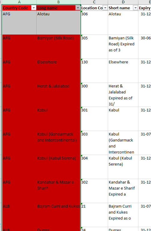
i have an excel sheet with 3000 rows with column A named countries and another column B named cities. I need to highlight the duplicate city names in column B for each country in column A and sort the data to show duplicates one after another. The city names have the same cell values but have additional information in parenthesis, and this is proving to be tougher to highlight the duplicates as excel is treating them as unique values. Below is the sample data. I would greatly appreciate if you could help me with a solution.

AFG	Alotau
AFG	Bamiyan (Silk Road)
AFG	Elsewhere
AFG	Herat & Jalalabad
AFG	Kabul
AFG	Kabul (Gandarmack and Intercontinental)
AFG	Kabul (Kabul Serena)
AFG	Kandahar & Mazar e Sharif

[#2]

@subbucat 

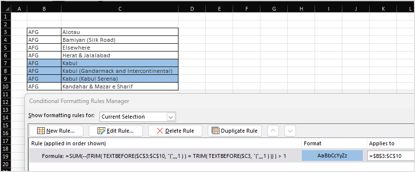
As variant, if you are on 365 or 2021

with

=SUM(--(TRIM( TEXTBEFORE($C$3:$C$10, "(",,,1 ) ) = TRIM( TEXTBEFORE($C3, "(",,,1 ) )) ) > 1

[#3]

Pro plus 2021

[#4]

@subbucat 

If above doesn't work you may try

=SUMPRODUCT(--(TRIM(  IFERROR( LEFT($C$3:$C$10, SEARCH("(",$C$3:$C$10)-1 ), $C$3:$C$10) ) = TRIM(  IFERROR( LEFT($C3, SEARCH("(",$C3)-1 ), $C3) ) ) ) > 1

[#5]

@Sergei Baklan I tried the 2nd formula and almost all rows got highlighted, except few. (The first one did not work). Thank you for helping

 

[#6]

@subbucat 

That's hard to comment without seen conditional formatting rule formula and range to which it applied. Finally desirably to see exact values for which the rule doesn't work.

[#7]

I made the changes to the formula

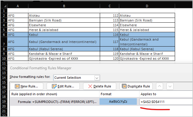
=SUMPRODUCT(--(TRIM( IFERROR( LEFT($B$2:$C$4111, SEARCH("(",$B$2:$B$4111)-1 ), $B$2:$B$4111) ) = TRIM( IFERROR( LEFT($B2, SEARCH("(",$B2)-1 ), $B2) ) ) ) > 1

[#8]

@subbucat 

At least it shall be

...LEFT($B$2:$B$4111)

[#9]

@Sergei Baklan Thank you. This has cleared the problem upto an extent. But now it is searching the whole sheet with all columns. whereas my search should be limited to A and B Columns.

ALB

Gjirokastra -Expired as of XXXX

112

Gjirokastra -Expired as of XXXXXX

Technically this is not duplicate but it is highlighting as duplicate because the same name exits in Column D.

[#10]

@subbucat 

Nope, it highlights entire row within the range if duplicate is in column B only. Here is the sample with your formula as in previous post