- Home
- Microsoft 365
- Excel
- Counting by referencing multiple tables in a single function.
Counting by referencing multiple tables in a single function.
- Subscribe to RSS Feed
- Mark Discussion as New
- Mark Discussion as Read
- Pin this Discussion for Current User
- Bookmark
- Subscribe
- Printer Friendly Page
- Mark as New
- Bookmark
- Subscribe
- Mute
- Subscribe to RSS Feed
- Permalink
- Report Inappropriate Content
Mar 08 2024 05:48 AM
Hello,
I'm having troubles figuring out the proper process to count the number of trades that are off on a certain date, using the following tables.
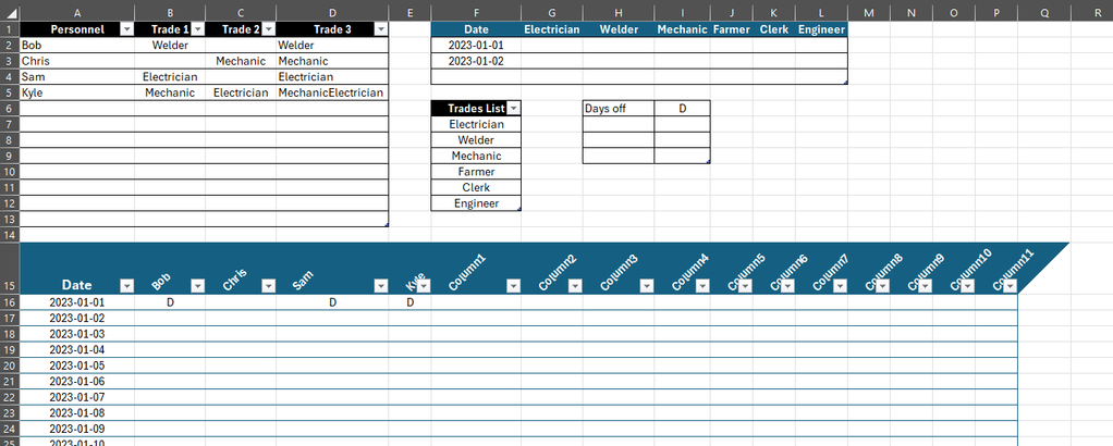
There is a table for the Personnel, linked to their trade (A1:D13), which limits their trade selection to a table of trades (Trade List).
There is a table for the days off a person has scheduled, where their days off are listed as a variety of symbols at the intersection of their name and date - currently only D is listed for Days Off (A15:P...). This will be the primary entry table that will be updated throughout the year.
Finally, there is the output table, that lists the trade against a date, and shows how many of each trade are off that date (F1:L4).
This output table would ideally remain a table to allow filtering by the date, but any other table can be switched to a range if it helps facilitate the process. I image some form of countifs would be required, but I'm admittedly fairly new to working with ranges and arrays for counting, especially when it's referencing multiple.
To summarize, I'm hoping for the final table to count the number of electricians off based on the date in the F column, by looking at the employees with the trade designation in the header, and then searching the days off table for a letter in the intersecting column. We would like to avoid power query or macros if possible. Any advice would be greatly appreciated!
Thanks,
- Labels:
-
Excel
-
Formulas and Functions
- Mark as New
- Bookmark
- Subscribe
- Mute
- Subscribe to RSS Feed
- Permalink
- Report Inappropriate Content
Mar 08 2024 06:50 AM
Could you please clarify a bit
Personnel Trades. For example Bob has Welder as Trade 1 and same Welder as Trade 3. Why so ? And, if some reason, Bob is "doubled Welder" and he is off on Jan 1st, does that mean we have TWO Welders off for that date.
Output. That will be much better of in your sample you add as well manually calculated result. Now it is empty in sample.
Input. How critical is such layout of ranges, they are not optimal. If for some reason (which one) we can't use unpivoted layout most probably we shall be do that in formulae and/or helper ranges.
If you'd like to avoid data modelling and PivotTables, which kind of formulas are available in your environment, are you on Excel 365?
- Mark as New
- Bookmark
- Subscribe
- Mute
- Subscribe to RSS Feed
- Permalink
- Report Inappropriate Content
Mar 08 2024 07:11 AM
Apologies for not explaining the personnel/trade table. The first two columns represent their two disciplines. They would always have a minimum of one, but may have two. The third table is just a concatenate I did to try and simply the functions by searching for partial matches, but forgot to remove before posting this. So if they are a welder and mechanic, one of each would be listed as off that day.
As for the output, see below pertaining to the example screenshot I gave;
Since Bob (Welder), Sam (Electrician), and Kyle (Mechanic and Electrician) are all off on that day, you have two electricians, one welder, and one mechanic off.
Also, no the range layout doesn't matter, it's just important that the personnel/date table is vertical.
I'm on the latest version of excel and Microsoft 365, and have access to all formulas, I'm just looking to avoid query and macros to simply the process - it's fairly important it's executed using only functions.
Hope this makes sense,
- Mark as New
- Bookmark
- Subscribe
- Mute
- Subscribe to RSS Feed
- Permalink
- Report Inappropriate Content
Mar 08 2024 07:26 AM
- Mark as New
- Bookmark
- Subscribe
- Mute
- Subscribe to RSS Feed
- Permalink
- Report Inappropriate Content
Mar 08 2024 07:54 AM
I see, thank you. If change the input a bit it could be like
with formulae as
=LET(
 nDates, 3,
 nTrades, COUNTA(Trades[Trades]),
 dates, SEQUENCE(nDates,,DATE(2023,1,1) ),
 header, TOROW(Trades[Trades],3),
 offDays, LAMBDA(date,trade,
   LET(
     offNames, FILTER(DaysOff[[Person]:[Person]],
        DaysOff[[Date]:[Date]]=date),
     tradeNames, FILTER(PeopleTrades[[Personnel]:[Personnel]],
        PeopleTrades[[Trade]:[Trade]]=trade),
     IFERROR(SUM(--(offNames=TRANSPOSE(tradeNames) ) ), 0)
 ) ),
 fillOff, MAKEARRAY(
    nDates,
    nTrades,
    LAMBDA(n,m,
      offDays(
          INDEX( dates,n,1),
          INDEX( header,1,m) ) )
  ),
 VSTACK(
    HSTACK( "Date", header ),
    HSTACK( dates, fillOff ) )
)
If such input is not desirable when transpose to like form within calculations.
- Mark as New
- Bookmark
- Subscribe
- Mute
- Subscribe to RSS Feed
- Permalink
- Report Inappropriate Content
Mar 08 2024 08:18 AM
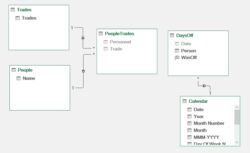
If to build PivotTable we need to add source data to data model first. Better to do that with Power Query, but if source tables do not require any transformations that could be done directly.
Also directly in Power Pivot or by Power Query to add Data (aka Calendar) table which covers dates for all desired periods.
Relationships could be set as
Measure to use
WasOff:=CALCULATE(
   COUNTROWS(  DaysOff ),
   TREATAS( VALUES(PeopleTrades[Personnel]), DaysOff[Person] )
 )
Resulting PivotTable looks like
- Mark as New
- Bookmark
- Subscribe
- Mute
- Subscribe to RSS Feed
- Permalink
- Report Inappropriate Content
Mar 08 2024 08:24 AM
- Mark as New
- Bookmark
- Subscribe
- Mute
- Subscribe to RSS Feed
- Permalink
- Report Inappropriate Content
Mar 08 2024 09:58 AM
Both do not require VBA.
First one is regular formula which uses Excel 365 function. You may copy/paste that formula in formula bar (or check it in the attached file) and it shall work. Since that's multiline formula better to expand formula bar.
Second one uses data model which shall be available practically on any more or less modern version of Excel Desktop. On Windows, not on Mac. Here is also no VBA coding. Tools to work with data model (build relationships, add measures) are within Excel.
- Mark as New
- Bookmark
- Subscribe
- Mute
- Subscribe to RSS Feed
- Permalink
- Report Inappropriate Content
Mar 08 2024 04:06 PM


