- Home
- Microsoft 365
- Excel
- Re: Apply different date filters to specific column values in a pivot table
Apply different date filters to specific column values in a pivot table
- Subscribe to RSS Feed
- Mark Discussion as New
- Mark Discussion as Read
- Pin this Discussion for Current User
- Bookmark
- Subscribe
- Printer Friendly Page
- Mark as New
- Bookmark
- Subscribe
- Mute
- Subscribe to RSS Feed
- Permalink
- Report Inappropriate Content
Feb 02 2022 10:55 AM
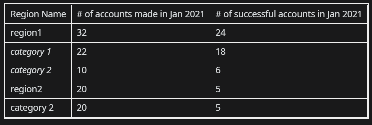
Suppose I have the following pivot table from one data source
The source data is essentially a spreadsheet of accounts which indicates 3 items (3 columns)- date account was created, date account was successful, date account was bought.
There are 3 stages an account goes through: step 1 it gets created. Step 2, if the employee deems the account to be successful, they mark it as successful and mark the date it became successful. If there is more interest in the account, the account is bought and the company receives money for it - they mark the date it was bought.
If you look at the data, the # of created accounts > # of successful accounts > # of bought accounts.
However, a created account can be made in Jan 2021 for example, but can be successful in Feb 2021 and then bought in June 2021. An account cannot necessarily be created, be successful, and be bought all in the same month/year.
That's the problem I have with this pivot table - the values field I have is using the count of date created, count of date successful and the columns on my pivot table is grouped by quarters of Y2021. The rows of the pivot table are the different regions the account belongs to. The problem I have is I am grouping the dates based on the date created and data is being filtered strictly from that date created filter; I don't know how to create a "global" date filter that is not strictly based on the date created filter
So, in the February 2021 column for example, it is telling me I have 8 created accounts and 6 successful accounts, when there really should be 5 successful accounts. If you double click that cell which launches a table of that data, you'll see an account that was successful in August 2021, however, it was created in February 2021, so that is why it will say 6 successful accounts . That is an example of a discrepancy in my pivot table. If region3 has 10 created accounts in January 2021 for example, and in the same month/year, has 5 successful accounts (by looking at the source data) and one account becomes successful in July 2021, the pivot table should indicate that correctly as 10 created accounts in Jan 2021 and 5 successful accounts in January 2021.
- Labels:
-
BI & Data Analysis
-
Excel
-
Office 365
- Mark as New
- Bookmark
- Subscribe
- Mute
- Subscribe to RSS Feed
- Permalink
- Report Inappropriate Content
Feb 02 2022 12:45 PM
@tytds
not sure I understood entire logic. For such sample
- creating PivotTable add data to data model
- add Date (Calendar) table with PowerPivot or Power Query
- make relationship between it and main table on Date <=> Made
- add measures as
accounts made:=COUNTROWS ( Table1 )

accounts success:=VAR mindate =
    MIN ( 'Calendar'[Date] )
VAR maxDate =
    MAX ( 'Calendar'[Date] )
RETURN
    CALCULATE (
        COUNTA ( Table1[Success] ),
        'Calendar'[Date] >= mindate
            && 'Calendar'[Date] <= maxDate
    )


accounts bought:=VAR mindate =
    MIN ( 'Calendar'[Date] )
VAR maxDate =
    MAX ( 'Calendar'[Date] )
RETURN
    CALCULATE (
        COUNTA ( Table1[Bought] ),
        'Calendar'[Date] >= mindate
            && 'Calendar'[Date] <= maxDate
)- Mark as New
- Bookmark
- Subscribe
- Mute
- Subscribe to RSS Feed
- Permalink
- Report Inappropriate Content
Feb 02 2022 12:49 PM - edited Feb 02 2022 12:52 PM
The columns would be months on the pivot table and there would be different years as the row labels
Also, your pivot table above is not accurate (there should be 0 successful accounts in Jan 2021)
- Mark as New
- Bookmark
- Subscribe
- Mute
- Subscribe to RSS Feed
- Permalink
- Report Inappropriate Content
Feb 02 2022 12:53 PM
- Mark as New
- Bookmark
- Subscribe
- Mute
- Subscribe to RSS Feed
- Permalink
- Report Inappropriate Content
Feb 02 2022 02:40 PM
- Mark as New
- Bookmark
- Subscribe
- Mute
- Subscribe to RSS Feed
- Permalink
- Report Inappropriate Content
Feb 03 2022 11:49 AM
If to continue it's better if you generate small sample file to illustrate the logic manually adding desired result. That's 5-10 minutes job, your actual data is not required.
- Mark as New
- Bookmark
- Subscribe
- Mute
- Subscribe to RSS Feed
- Permalink
- Report Inappropriate Content
Feb 03 2022 12:14 PM
https://easyupload.io/zlogle
- Mark as New
- Bookmark
- Subscribe
- Mute
- Subscribe to RSS Feed
- Permalink
- Report Inappropriate Content
Feb 04 2022 05:35 AM
@tytds
thank you, but that doesn't explain the logic. In sample file we have 12 accounts submitted in January. Each of them has Date Successful, thus all 12 of January accounts are successful.
Or you mean count successful accounts only if Date Successful is in January, doesn't matter when they were submitted?
Or some other logic?
- Mark as New
- Bookmark
- Subscribe
- Mute
- Subscribe to RSS Feed
- Permalink
- Report Inappropriate Content
Feb 04 2022 05:02 PM
- Mark as New
- Bookmark
- Subscribe
- Mute
- Subscribe to RSS Feed
- Permalink
- Report Inappropriate Content
Feb 05 2022 04:27 AM
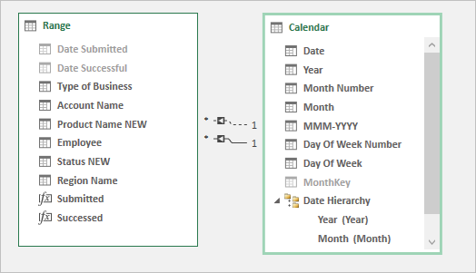
With that you need to create separate Date (aka Calendar) table. That could be done by Power Query or directly in PowerPivot. Make relationships with main table and hide date fields in the latest.
Create measures
Submitted:=CALCULATE (
    COUNTROWS ( Range ),
    USERELATIONSHIP ( 'Calendar'[Date], Range[Date Submitted] )
)
and
Successed:=CALCULATE (
    COUNTROWS ( Range ),
    USERELATIONSHIP ( 'Calendar'[Date], Range[Date Successful] )
)
use them in PivotTable
- Mark as New
- Bookmark
- Subscribe
- Mute
- Subscribe to RSS Feed
- Permalink
- Report Inappropriate Content
Feb 05 2022 10:50 PM
- Mark as New
- Bookmark
- Subscribe
- Mute
- Subscribe to RSS Feed
- Permalink
- Report Inappropriate Content


