Urgent help: How to use VLOOKUP function?

[helis430]

Hi guys,

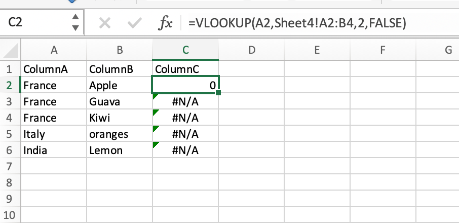
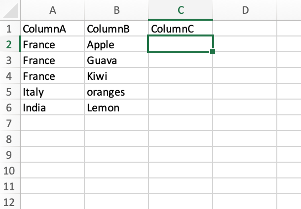
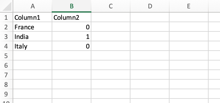
I have been trying to extract the values for a column from sheet2 using the name as the VLOOKUP value in sheet 1. Unfortunately, it is only working for few records and for most of the records, it is just giving me #N/A values. According to my understanding, it might be because the same VLOOKUP names are appearing more than once in sheet1 because sheet1 contains data about multiple items belonging  to the same VLOOKUP name due to which the same VLOOKUP name is appearing multiple times.

I would really really appreciate some guidance.

[#2 · Accepted solution]

@helis430 Can you at least provide the formula you are using and confirm that Sheet2 is in the top picture and Sheet1 in the bottom? If you could upload the file, that would be even better. Remove any confidential information though.

[#3]

Hello @Riny_van_Eekelen,

Thanks for the response!

The second screenshot is an example for the sheet1 and the third is for sheet2. The formula I am using in sheet1 columnC is:=VLOOKUP(A2,Sheet2!A2:B4,2,FALSE). And at the top is the screenshot of sheet1 after applying the formula. These three examples of the sheets represent the issue I am facing.I would really appreciate some guidance on how to modify the VLOOKUP function further to avoid getting #N/A values. The function has given me the right value just for the first row, whereas sheet2 has values for all the VLOOKUP values. I am very stuck.

[#4]

@helis430 I suspect that you just copied down that formula. Change it to:

=VLOOKUP(A2,Sheet2!$A$2:$B$4,2,FALSE)

This will fix the reference to the lookup array. when you leave out the $ signs and copy down, the reference will become A3:B5, A4:B6 and so on. Then VLOOKUP finds no matches, hence #NA.

Better to use structured table references or named ranges. For instance, create a named range called "lookuptable" referring to Sheet2!$A$2:$B$4 and then change the formula to 

=VLOOKUP(A2,lookuptable,2,FALSE)

.. and you don't have to worry about the sheet name or the $ signs.

By the way, you write Sheet2, but the formula in your screenshot uses Sheet4.

[#5]

Hello @ Riny_van_Eekelen,
Thanks a ton!
It worked!!!!!!!!