Too many arguments error on IF/COUNTIF nested function: how to solve

[Vesperwind]

Hi all, 

I need to write an excel formula with way too many nested functions, like the following one, but much longer: 

=IF(COUNTIF(F7;"*Example A*");"A";IF(COUNTIF(F7;"*Example B*");"B";IF(COUNTIF(F7;"*Example C*");"C";IF(COUNTIF(F7;"*Example D*");"D";IF(COUNTIF(F7;"*Example E*");"E";IF(COUNTIF(F7;"*Example F*");"F";IF(COUNTIF(F7;"Example G*");"G";IF(COUNTIF(F7;"*Example H*");"H";"")))))))) etc. etc.

Obviously at some point, if I add more conditions I'll receive the following error: "You've entered too many arguments for this function". 

Now, since I absolutely need to write all those values to make the results appear on the one cell where I write the formula, is there a way to solve this problem? 

Thank you very much

[#2]

@Vesperwind 

Initial formula

=IF(
    COUNTIF(F7, "*Example A*"), "A",
    IF( COUNTIF(F7, "*Example B*"), "B",
    IF( COUNTIF(F7, "*Example C*"),"C",
    IF(COUNTIF(F7, "*Example D*"),"D",
    IF( COUNTIF(F7, "*Example E*"), "E",
    IF( COUNTIF(F7, "*Example F*"), "F",
    IF( COUNTIF(F7, "Example G*"), "G",
    IF(COUNTIF(F7, "*Example H*"), "H",
         "")
    )  ) )  ) ) ) )

works correctly. Which formula doesn't work?

[#3 · Accepted solution]

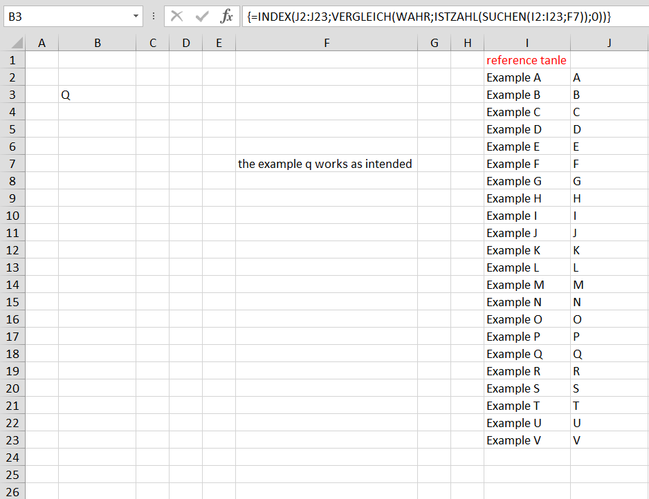
@Vesperwind 

=INDEX(J2:J23,MATCH(TRUE,ISNUMBER(SEARCH(I2:I23,F7)),0))

An alternative could be this formula along with a reference table. Enter the formula with ctrl+shift+enter if you don't work with Office 365 or Excel 2021. The formula is in cell B3.

[#4]

Hey @OliverScheurich! Sorry for the late reply!
I'd like to thank you because your formula works pretty well!!!
The only very last problem I have is when the F7 cell is empty: I get "#N/D" on B3.
Since when you open my file the starting point is you have 0 conditions applied, it would be visually good to have an empty cell instead of "#N/D".
Is there any solution to apply this in the formula? Otherwise I would go for conditional formatting...

[#5]

@Vesperwind 

You are welcome. Glad the formula works almost as intended.

=IFERROR(INDEX(J2:J23,MATCH(TRUE,ISNUMBER(SEARCH(I2:I23,F7)),0)),"")

In order to return an empty cell B3 if F7 is empty you can try this formula. Actually i've only wrapped the formula into IFERROR. The formula has to be entered with ctrl+shift+enter if one doesn't work with Office 365 or Excel 2021.

[#6]

That's what I needed!
Thank you SO much @OliverScheurich!!!!