Problem with Conditional Formatting that have Formula

[oayrancioglu]

Hi everyone,

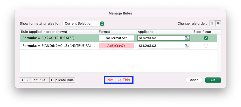
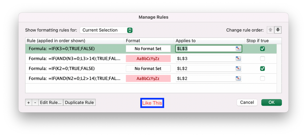
I made an IF statement as a formula for "conditional formatting" and I try to apply that "conditional formatting" for each cell by avoiding merge that "conditional formatting". Everytime I tried to use "format" button to copy that "conditional formatting" into the next cell below, it keeps the formula still but applying that formula to that two cells. I need the formula in "conditional formatting" change relatively while changing cell.. So what I mean to say that is it possible to use that "conditional formatting" for each cell individually by adapting the formula in it into cells automatically? Like in the screenshot I shared with you. Also I'll use this format for almost 5000 cell.. So it can't be done manually..

It should not be like thisIt should be like this

Thank you for taking time to help me.

Oguzhan

[#2 · Accepted solution]

@oayrancioglu 

You should use rules as in the "not like this" screenshot.

Since the formulas in the rules use relative cell references, Excel will automatically adjust them for each cell in the 'Applies to' range, regardless of how large that range is.

By the way, it isn't necessary to explicitly use IF with TRUE and FALSE in the formulas.

=IF(K2=0;TRUE;FALSE)

is equivalent to

=K2=0

and

=IF(AND(N2=0;L2>14);TRUE;FALSE)

is equivalent to

=AND(N2=0;L2>14)

[#3]

@Hans Vogelaar 

“Excel will automatically adjust them for each cell in the 'Applies to' range, regardless of how large that range is.”

As I mentioned before that does not help. Excel won’t change the cell numbers automatically regarding to based cell number. As you can see on the screenshot of “Not like this”, K, N and L are still in contrast to “apply to” cell changes. So If I leave it like this, “apply to” cells always check conditions in the cells of K2, N2 and L2. I need these conditions to be adjust relatively according to “apply to” cells..

Also, I thank you for the tips about IF statement. 

[#4]

@Hans Vogelaar and @oayrancioglu

It was my mistake. It's pretty complicated worksheet that I am working on so my references mixed up by me. As you said It's working well. It is adjusting itself automatically even if cell numbers don't change in the conditional formatting window. Thank you very much again.
Best wishes
Oguzhan