Need help with creating a formula

[RyanC1990]

Still learning more complex formulas with excel, so some help would be appreciated with some steps to make this happen.

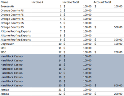
I'm trying to process a large group of data to come up with a few different things for some reporting. I want to have column D generate the sum total from column C, for all invoices that share the same name in column A, and have that sum appear on the cell of the last row the name appears on. This needs to be continuing for the entire spreadsheet.

Additionally, I need some conditional formatting that where names that exceed the sum total of $500 to highlight in a color so I can then filter by color later on. Please reference the screenshot below, anyone able to assist with something like this?

Appreciate everyone! 

[#2]

@RyanC1990 

=SUMIF($A$2:$A$23,$A2,$C$2:$C$23)>500

You can apply this rule for conditional formatting.

=$A$2:$D$23

This is the range the conditional format applies to.

=IF(COUNTIF($A$2:A2,A2)=COUNTIF($A$2:$A$23,A2),SUMIF($A$2:A2,A2,$C$2:C2),"")

This formula returns the results in column D.

[#3]

@RyanC1990 

A 365 solution. The key is finding when the account name changes.  The attached workbook contains your sample data. Ranges are dynamic.

=LET(
    acct_change, XMATCH(UNIQUE(Name), Name, , -1) + 1,
    AcctTotal, LAMBDA(n, IF(XOR(ROW(n) = acct_change), SUMIF(Name, n, InvoiceTotal), "")),
    MAP(Name, AcctTotal)
)

[#4]

To achieve this in Excel, use the SUMIF formula in column D to sum values from column C based on the names in column A. In cell D2, enter =IF(A2<>A1, SUMIF(A:A, A2, C:C), "") and drag it down. This will display the sum only in the last row for each name. For conditional formatting, select column D, go to Home > Conditional Formatting > New Rule, and use the formula =D2>500 to highlight cells where the sum exceeds $500.