If And Formula

[CatherineMadden]

I have a sheet that I want a formula to return a value if a name and date are found. This is going to need to work on a larger scale, this is just a small example. 

[#2]

I'm going to guess that each person has a table below their name and each table has those same dates so it isn't IF you find that name it is more about finding a date in a table that is directly under that name. That said I would recommend inserting a column to the left or right of the table with a simple formula like the following assuming you insert the column at A and this goes into (the new) A2 and you fill down

=IF(L7="Date", L6, K6)

(remember after you insert a column to the left of the table the name and Dates will be in column B)

now you could use a pivot table to create that table or various lookup techniques like:

=FILTER($M:$M, ($K:$K=$R2)*($L:$L=S$1), "")

or

=SUMIFS($M:$M, $K:$K, $F3, $L:$L, G$2)

You can also do this all in a single formula like:

=LET(in,K6:L26,people,Q2:Q4,Dates,R1:S1,
name,SCAN("",SEQUENCE(ROWS(in)),LAMBDA(p,q,IF(INDEX(in,q,1)="Date",INDEX(in,q-1,1),p))),
MAKEARRAY(ROWS(people),COLUMNS(Dates),LAMBDA(r,c,FILTER(TAKE(in,,-1),(name=INDEX(people,r))*(TAKE(in,,1)=INDEX(Dates,c)),""))))

EDIT: I editted the above formula based on the file you attached and updated the file (see attached).  In the attached the 1st sheet I inserted the extra column and on the second sheet I used the LAMBDA function to do it all.

[#3]

@CatherineMadden 

Certainly! To create a formula that returns a value based on two conditions – finding a specific name and date – you can use the IF AND function in Excel. Here's how:

Formula structure:

Excel=IF(AND(criteria1, criteria2), value_if_true, value_if_false)

Explanation:

• criteria1 and criteria2: These represent the individual conditions you want to check. These can be cell references, comparisons, or other logical expressions.
• value_if_true: This is the value returned if both criteria1 and criteria2 are true.
• value_if_false: This is the value returned if either criteria1 or criteria2 is false.

Example:

Suppose you have a table with names in column A and dates in column B. You want a formula in cell C2 to return "Found" if the name in cell A2 exists and the date in cell B2 is after March 1, 2024. Here's the formula:

Excel=IF(AND(A2="John Doe", B2>DATE(2024,3,1)), "Found", "")

This formula checks if:

• The name in A2 matches "John Doe" (replace with your actual name)
• The date in B2 is greater than March 1, 2024

If both conditions are true, it returns "Found"; otherwise, it returns an empty string ("").

Tips:

• You can use cell references or direct values for your criteria.
• You can nest multiple IF AND functions for more complex conditions.
• Consider using error handling functions like ISNA or IFERROR to handle potential errors like missing data.

Remember:

• Adapt the formula to your specific table layout and conditions.
• Adjust the value_if_true and value_if_false based on your desired outputs.

I hope this helps

[#4]

@smylbugti222gmailcom 

Attached is a small example of the data. They are in the same Rows/Columns so when I transfer the formula, I shouldn't have to make any changes.

I need this formula to auto fill down and to the right.

[#5]

see updates made to my comment above

[#6]

@CatherineMadden 

There are some good formula responses here, so let me add a Power Query response. 

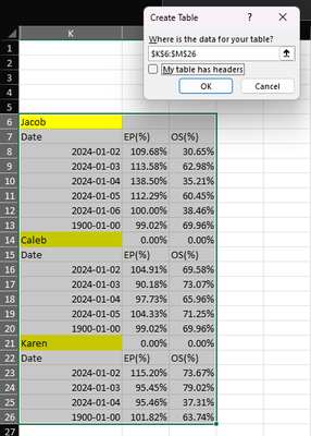
First, select the data range then use Data > Get & Transform Data > From Table/Range, ensuring that 'My table has headers' is not checked, like this:

After you click OK, the Power Query editor will open:

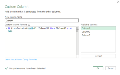
Use Add Column > Add Custom Column and configure it like this:

if List.Contains({null,0},[Column2]) then [Column1] else null

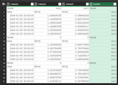
Which gives you this:

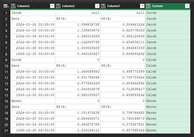
Now select the 'Custom' column and right-click and select Fill > Down to get this:

Now change the data type of Column1 to Date. Click the ABC123 icon in the column header:

This gives you:

Now with Column1 still selected, use Home > Remove Rows > Remove Errors:

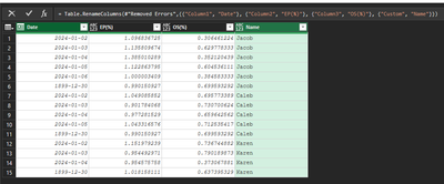
Now double-click each column and rename them appropriately:

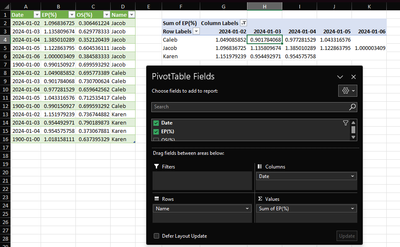
Now use Home > Close & Load , then create a pivot table:

Now you can restructure the pivot table however you want, or create another summary. Additionally, this query can be re-run whenever there are changes to the source data.