How to check if all cells in a non congruent range/list meet specific criteria. See below.

[spinaz0070]

I am trying to use the following formula to see if 1. All 39 cells in row C have data, 2. All cell values are greater than 225, and 3. All cell values are less then 384.  If all conditions are met, then it should populate PASS, otherwise FAIL.  This formula is not working, and pretty sure it's because of my countif statements, but just not sure how to do this.
Any help is appreciated!

Scott

=IF(AND(COUNTA(C17,C19,C21,C23,C25,C27,C29,C31,C33,C35,C37,C39,C41,C43,C45,C47,C49,C51,C53,C55,C57,C59,C61,C63,C65,C67,C69,C71,C73,C75,C77,C79,C81,C83,C85,C87,C89,C91,C93)=39,COUNTIF(C17,C19,C21,C23,C25,C27,C29,C31,C33,C35,C37,C39,C41,C43,C45,C47,C49,C51,C53,C55,C57,C59,C61,C63,C65,C67,C69,C71,C73,C75,C77,C79,C81,C83,C85,C87,C89,C91,C93)>=225,COUNTIF(C17,C19,C21,C23,C25,C27,C29,C31,C33,C35,C37,C39,C41,C43,C45,C47,C49,C51,C53,C55,C57,C59,C61,C63,C65,C67,C69,C71,C73,C75,C77,C79,C81,C83,C85,C87,C89,C91,C93)<=384),"PASS","FAIL")

[#2]

@spinaz0070  I'm sure it's possible to come up with a more elegant solution than this. But as a pointer to you in terms of developing a formula that can work, you might try -- as I've done in the attached --with a smaller set of cells replicating the condition you're looking for. Then when you get something that works, you could extend it. BUT, see my concluding comment at the bottom.

Here are shown the three formulas I've used that work for just three cells with disparate values. These could be combined into one that just checks to make sure each produces the full count showing that all satisfy your "PASS" criteria.

However, I wonder whether you couldn't redesign your sheet so that the values being checked ARE contiguous.....that would make more sense, in the long run. Even if there's some other process in the cells in the midst of these, you could have these crucial cells for the Pass/Fail in a different location, as a single range.

[#3]

@spinaz0070 

In my understanding all cells need to have values (condition 1) otherwise the values can't be greater than 225 (condition 2) and less than 384 (condition 3). If a cell doesn't have a value conditons 2 and 3 can't be true.

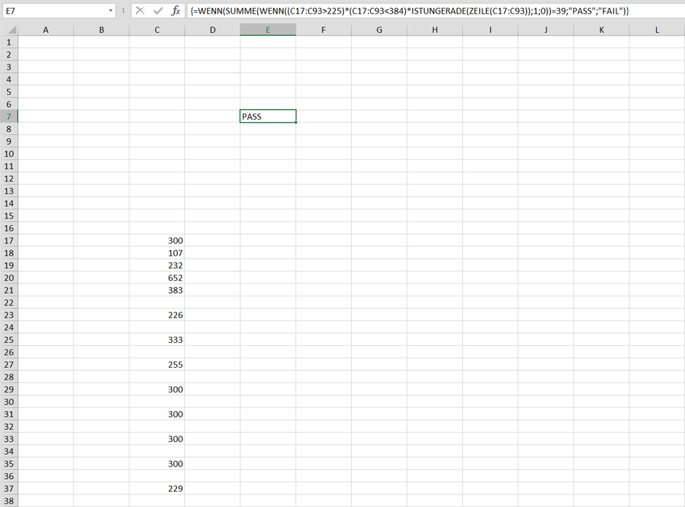
This formula checks for each uneven row if the cells in range C17:C93 have a value greater 225 and less than 384. If it is greater 225 and less than 384 the formula returns 1 otherwise 0. The SUM counts the 1s and 0s and the result must be 39 for the "PASS".

=IF(SUM(IF((C17:C93>225)*(C17:C93<384)*ISODD(ROW(C17:C93)),1,0))=39,"PASS","FAIL")

Enter the formula with ctrl+shift+enter if you don't work with Office 365 or Excel for the web or Excel 2021.

[#4]

Thanks Mathetes.
I thought about using a similar formula (e.g. IF(AND(C17>225,C19>225,...C17<384,C19<384,...),"PASS", "FAIL"), but I don't want to do this due to the number of cells (39).
I wish Microsoft would allow for non-congruent cells in their formulas, as I can't make mine congruent.
Appreciate your response!

[#5]

@spinaz0070 

I wish Microsoft would allow for non-congruent cells in their formulas, as I can't make mine congruent.

But you can create a range elsewhere (we refer to such things as "helper columns") that takes all the values in those odd numbered cells and puts them into a single continuous array.

[#6]

Hi Oliver. Can you please help me understand this formula. Why don't the first two conditions (>225, <384) need to call out the odd rows, and what do the ,1,0 do in the ISODD(ROW) condition? Just trying to learn the syntax. Thanks

[#7]

@spinaz0070 

{TRUE,FALSE,TRUE,FALSE,TRUE,FALSE,TRUE,FALSE,TRUE,FALSE,TRUE,FALSE,TRUE,FALSE,TRUE,FALSE,TRUE,FALSE,TRUE,FALSE,TRUE,FALSE,TRUE,FALSE,TRUE,FALSE,TRUE,FALSE,TRUE,FALSE,TRUE,FALSE,TRUE,FALSE,TRUE,FALSE,TRUE,FALSE,TRUE,FALSE,TRUE,FALSE,TRUE,FALSE,TRUE,FALSE,TRUE,FALSE,TRUE,FALSE,TRUE,FALSE,TRUE,FALSE,TRUE,FALSE,TRUE,FALSE,TRUE,FALSE,TRUE,FALSE,TRUE,FALSE,TRUE,FALSE,TRUE,FALSE,TRUE,FALSE,TRUE,FALSE,TRUE,FALSE,TRUE,FALSE,TRUE}

The above is the result of the evaluation of:

ISODD(ROW(C17:C93))

This means that the odd and even rows are determined by ISODD(ROW(C17:C93)) and this hasn't to be done again with the first two conditions.

This is the original formula.

=IF(SUM(IF((C17:C93>225)*(C17:C93<384)*ISODD(ROW(C17:C93)),1,0))=39,"PASS","FAIL")

This is the inner IF formula perhaps more readable with some spaces:

IF(  (C17:C93>225)*(C17:C93<384)*ISODD(ROW(C17:C93))    ,    1,      0)

The   ,    1,      0) aren't within the ISODD(ROW)  condition.

Within IF this

(C17:C93>225)*(C17:C93<384)*ISODD(ROW(C17:C93))

is the condition which is checked and if it's true then 1 is returned and if false 0 is returned.

Below is what the evaluation of 

IF(  (C17:C93>225)*(C17:C93<384)*ISODD(ROW(C17:C93))    ,    1,      0)

returns in the formula bar.

[#8]

@spinaz0070 

I offer a 365 solution:

=LET(
    rng, C17:C93,
    wrapped, WRAPROWS(rng, 2, ""),
    vector, TOCOL(TAKE(wrapped, , 1), 1),
    tally, COUNT(vector),
    total, SUM(vector),
    IF(AND(tally = 39, total > 225, total < 384), "Pass", "Fail")
)

[#9]

@Patrick2788 

Thank you for that solution!

I had wondered if there was a way to create a vector like that, using LET and a couple  of intervening steps. I've never used those three functions--WRAPROWS, TOCOL and TAKE.

Thanks for showing the how to.