help

[Ginalea1610]

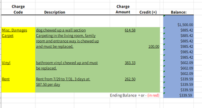
Can someone please help me figure out how to do this? I am trying to get the column in blue to have a running total of deductions and credits from a total starting amount, and the end result at the bottom...which I have! Yay me.  I know this is the easy part! 

Can someone help me to make the blue cells be empty UNLESS there was a change in that row which would result in a new number being generated? Basically the numbers of the running total would not repeat if they are not different.  So in the picture below, the  green highlighted cells would just be blank! I have no idea how do do this.

Thank you all for help in the past, you've been great!!

[#2 · Accepted solution]

@Ginalea1610 

Let's say the starting balance is in H5, the Charge Amounts in E6 and down, and the Credit Amounts in F6 and down.

In H6:

=IF(AND(E6:F6=""), "", $H$5-SUM(E$6:E6)+SUM(F$6:F6)

Fill down.

[#3]

@Ginalea1610 

=IF(AND(C3="",D3=""),"",INDEX($E$2:E2,LARGE(IF($E$2:E2<>"",ROW($E$1:E1)),1))-C3+D3)

An alternative could be this formula. Enter the formula with ctrl+shift+enter if you don't work with Office 365 or Excel 2021.

[#4]

@Ginalea1610 

This is more of a small essay than concise formula"

= LET(
    transaction,  credit-debit,
    runningTotal, SCAN(initialBalance, transaction, ADDλ),
    VSTACK(
      IF(transaction<>0, runningTotal, ""),
      SUM(initialBalance, credit, -debit)
    )
  )

where
ADDλ
= LAMBDA(x, y, x+y)