** HELP ** Need to return multiple results/values

[sruk89]

Hi,

Not sure what is best to use here, XLOOKUP, INDEX & MATCH or FILTER but i need help

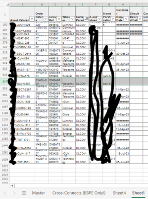
What I'm looking to achieve is return multiple values on tab "Master" Column K "Open Orders" based on the codes based in Column B "Sites" however as we can see there can be one or multiples codes in Column B "Sites" which are separated by a comma "," and based on those values i want it to return the values found on tab "sheet 1", Column A "Asset Reference" (Image 2 below) in image 2 in Tab Sheet 1Column E "Current Parent" we can reference these codes against Column B "Sites" on tab "Master"

Image 1

Image 2

Any help is appreciated from anyone!

@HansVogelaar maybe you might know?

Regards,

Scott

[#2]

@sruk89 

In K2 on the Master sheet:

=TEXTJOIN(" / ",TRUE, XLOOKUP(TEXTSPLIT(B2,","),Sheet1!$E$2:$E$1000,Sheet1!$A$2:$A$1000,""))

Adjust the ranges if Sheet1 has more than 1000 data rows.

Fill down.

[#3]

@HansVogelaar ,

Thanks for this much appreciated, it doesn't appear to return all matches, please see below.

In this example in Column B "Sites" i have put "CLCOV" on sheet 1 (Image 2) i did a filter and it returns more than 1 (25 in fact) it only appears to return xxx-LUMN-026

Image 2

[#4]

@sruk89 

Could you attach a small sample workbook demonstrating the problem (without sensitive data), or if that is not possible, make it available through OneDrive, Google Drive, Dropbox or similar?

[#5]

Hi hans,

I sent you a DM with a link to a sample doc.

Look forward to your response :)

Thanks,

Scott

[#6]

@sruk89 

See the attached version. I created a small lambda function - see Name Manager on the Formulas tab of the ribbon - to be able to "or" a range row by row.

[#7]

Thanks @HansVogelaar  as always!

Can you walk me through how to do this on the actual sheet, these are completely new functions to me. Appreciate it!

[#8 · Accepted solution]

@sruk89 

Step 1:

On the Formulas tab of the ribbon, in the Defined Names group, click Define Name.

Enter OrRow in the Name box, and enter the formula =LAMBDA(r,OR(r)) in the Refers To box.

Click OK to save the name.

The LAMBDA Function is a relatively new function in Excel. It allows us to create custom functions. This is a very simple one: it ORs the values of the supplied range.

Step 2:

The formula in K2 on the Master sheet is

=TEXTJOIN(" / ",TRUE, FILTER(Sheet1[Asset Reference],BYROW(Sheet1[Current Parent]=TEXTSPLIT([@Sites],","),OrRow),""))

TEXTSPLIT([@Sites],",") splits the value of the Sites column in the same row with comma as delimiter.

So if Sites contains "MRBUX,MRCHA", TEXTSPLIT will return "MRBUX" and "MRCHA" as separate values.

Sheet1[Current Parent]=TEXTSPLIT([@Sites],",") compares the Current Parent column of Sheet1 to these values. It returns TRUE for each match, FALSE for each mismatch.

In the above example, where TEXTSPLIT returns 2 values, Sheet1[Current Parent]=TEXTSPLIT([@Sites],",")  returns 2 columns of TRUE/FALSE values.

Normally, OR tests ALL cells in a range and returns one result. Here, however, we want to test row by row. We want to return a row if either of the values returned by TEXTSPLIT in that row is TRUE (a match).

We use the new BYROW Function for this purpose. We feed it Sheet1[Current Parent]=TEXTSPLIT([@Sites],",") and apply our custom function OrRow to it.

The result is ONE TRUE/FALSE value per row.

FILTER(Sheet1[Asset Reference],BYROW(Sheet1[Current Parent]=TEXTSPLIT([@Sites],","),OrRow),"")

filters the Asset Reference column on Sheet1 and returns only the rows for which BYROW(...) returns TRUE.

Finally, TEXTJOIN concatenates the result with " / " as delimiter.

[#9]

@HansVogelaar,

Thanks for explaining, much appreciated!

I have entered in the info as mentioned but I'm getting the following error:

[#10]

@sruk89 

Which version and build of Office do you have? You can check it by selecting File > Account. This is what I see:

[#11]

@HansVogelaar.,

When i open your sample doc you sent me it works fine, however when i try to copy what you've done, it doesn't seem to let me.

[#12]

@sruk89 

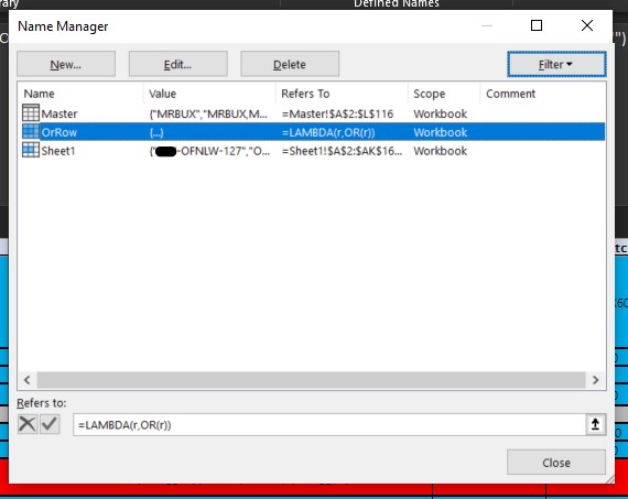
Which formula do you see for OrRow in Name Manager (on the Formulas tab of the ribbon) in my version of the workbook?

[#13]

@HansVogelaar ,

This is what can be seen in your version:

This is what is in my version:

The only difference i can see is what i've highlighted in the red circle, not sure whether this would have any significance?

[#14]

@HansVogelaar 

Phase 2b Pilot Scenarios.xlsx - here is the actually file, I have removed the sensitive data.

Regards,

Scott

[#15]

@sruk89 

Yes, that difference is relevant. In the earlier version, Sheet1 contained a table of the same name; in your "real" workbook, Sheet1 does not contain a table. I converted the data on Sheet1 to a table, and used its name (Table1 was assigned by Excel, but you can change it if you prefer) in the formula.

[#16]

@HansVogelaar ,

Ahhh yes, now i see. I have now done that and it works fine!

Thank you so much for you help, patience and time Hans!