** HELP ** Conditional Formatting

[sruk89]

Hi All,

Conditional formatting is by far my worse ability in Excel

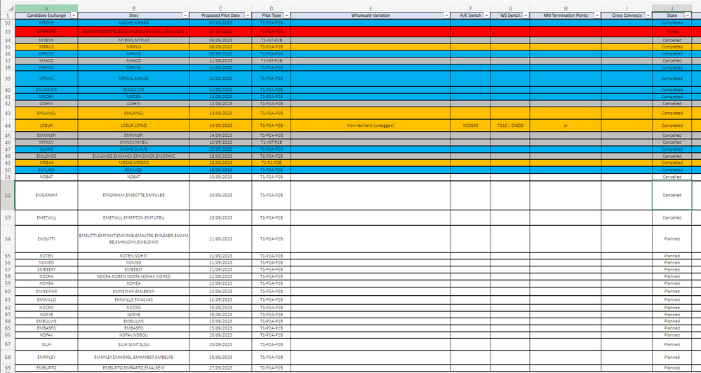
What im looking to achieve is if the Column J "State" Contains Complete or Completed i'd like the entire row to be Blue. If it says Cancelled, Grey, if Failed, red

@Sergei Baklan - maybe you can help me again 

Thanks in advance.

Regards,

Scott

[#2 · Accepted solution]

@sruk89 

Select all the rows that you want to format this way.

I'll assume that row 2 is the top row in the selection.

The active cell in the selection should be in that top row.

On the Home tab of the ribbon, click Conditional Formatting > New Rule...
Select 'Use a formula to determine which cells to format'.
Enter the formula

=OR($J2="Complete",$J2="Completed")

Click Format...
Activate the Fill tab.
Select blue as highlight color.
Click OK, then click OK again.

Repeat these steps, but with the formula

=$J2="Cancelled"

and grey as fill color.

Finally, repeat them again with

=$J2="Failed"

and red.

[#3]

Thanks Hans, much appreciated.