Excel Lookup That Skips Cells

[Morbeus]

Hi all,

Been struggling with this problem that seems like it should be simple, but I suspect I don't know enough to figure out what combination of things would work.

To summarise the setup (simplified) I have two sheets, Sheet 1 has some data in Column A, and I want to put the lookup formula in Column B.

Sheet 2 has data in Column C and D, I want the formula to look up the value of the Sheet 1 A cell in Column D, then return the corresponding value in Column C. However, if the value is 0, I want the formula to look "up" to find the next non-0 cell and return that value.

So, the first bit is relatively simple, I can just do =XLOOKUP(A1, Sheet2!D:D, Sheet2!,C:C) and that takes care of looking up to the left. What I'm having trouble with is how to then go up to the next non-zero cell.

I've got a workaround for the moment where I use =IF(XLOOKUP(A2, Sheet2!D:D, Sheet2!,C:C)=0,B1,XLOOKUP(A2, Sheet2!D:D, Sheet2!,C:C))

Basically, if the lookup isn't 0 use that value, if it is then use the value in the cell above this one. This isn't ideal as it needs manual verification that it's correct, and relies on there being something in the cell above that makes sense.

So, I'm fairly sure I need to modify this IF() statement to do something more interesting when the lookup returns 0, but I've not been able to figure out what. If anyone has any thoughts, I'd be extremely grateful.

[#2]

@Morbeus 

As variant

=LET(f, FILTER(Sheet2!C:C, (Sheet2!D:D=A1) ), IFERROR( @FILTER( f, f<>0 ), "no such") )

[#3]

@Sergei Baklan
I'm afraid I can only half-follow what that formula is doing. Could you explain the logic?

Many thanks.

[#4]

@Morbeus 

We filter from column C in Sheet2 all values for which value in column D is equal to A1. Result is filtered on all non-zero values. From these non-zero values we take first found by applying "@". Finally, if nothing was found, IFERROR gives a message.

[#5]

@Sergei Baklan 

Thank you for the explanation.

Unfortunately, this doesn't seem to be working, in that it's returning the "no such" message. I may not have explained properly.

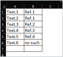
The columns look something like this on Sheet1:

   A              B     

Text.1     Formula

Text.2      Formula

Text.3      Formula

Text.4      Formula

Text.5      Formula

Text.6      Formula

On Sheet2:

  C            D

Ref.1         0

0           Text.1

0           Text.2

0               0

Ref.2     Text.3

Ref.3         0

0           Text.4

Ref.4     Text.5

In reality, there are other columns on the sheets between these with other data, but this is the setup for the ones I care about at the moment.

The idea is, look in each Sheet1 A cell, find where the value there is in the Sheet2 D column, then look to the left and return the value from the C column. If there's nothing there, then look "up" the column for the next non-zero entry and return that.

So, the formula in B1 and B2 looks at the values for A1 and A2 respectively and both should return "Ref.1", the formula in B3 should return "Ref.2", and so on.

When I apply the formula you kindly suggested to this example, I get the "no such" message on rows 1, 2, 4, and 6, i.e., wherever the Ref. is not immediately to the left of the Text.

Does that make the problem a little more clear?

[#6]

@Morbeus 

Does this do what you want?

=INDEX(Sheet2!C:C,XMATCH(TRUE,INDIRECT("Sheet2!C1:C"&MATCH(A1,Sheet2!D:D,0))<>0,0,-1))

You can wrap the INDEX formula in IFERROR to return something else instead of #N/A, of course

[#7]

@Hans Vogelaar
So, if I'm understanding this correctly, the inner MATCH function finds the position of the value from A in the D column, then the INDIRECT allows concatenation of that into the definition of the lookup range into the C column, and then the XMATCH function searches bottom-to-top in the C column range that's just been defined to find the correct Ref?

That's an excellent solution, thank you. I was convinced I was going to need nested IF() statements to handle the conditionals.

[#8]

@Morbeus 

Sorry, I misunderstood the logic. Close to what @Hans Vogelaar suggested

=LET(
 ref, Sheet2!C:C,
 txt, Sheet2!D:D,
 IF(A1="", "",
 IFNA(INDEX( ref,  XMATCH( XMATCH(A1,txt,0),ROW(ref)*(ref<>0),-1) ), "no such" ) ) )

[#9]

@Morbeus 

Yes, you have understood the formula correctly!