each letter of word in to separate cells

[Vimal_Gaur]

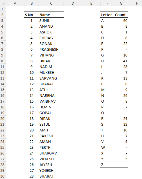
I need to extract the each letters of a word / words in to each separate cells.

(example attached)

or 

I need to count the occurrence in of a particular letters in a table.

(example attached)

the purpose is to know the number of each letter so that I can order printing quantity accordingly.

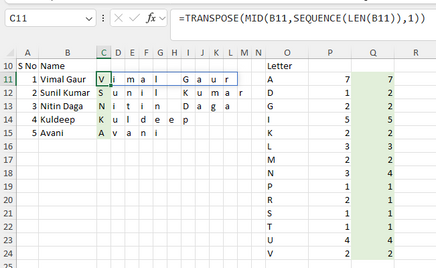
[#2 · Accepted solution]

@Vimal_Gaur Provided you are using Excel365 or 2021, have a look at the attached file.

The green shaded areas is where I entered my formulas.

[#3]

Thanks for reply.
I know the COUNTIF formula, I can do the counting myself.
I need to extract the letters in separate cells or if you can count the letters in the whole string.
e.g. 1. "Vimal Gaur" in a single cell B11 (find how many A are there in this word)
e.g. 2. "Rozer Ramon is lives right on bank of river" now find occurrence of each letter in this string.

[#4]

@Vimal_Gaur I merely replicated what was in your file. But WITH formulas. Did you note the formula in C11 and below? That's splitting each text string in B into separate cells. If that's not what you wanted, I misunderstood. 

[#5]

@Riny_van_Eekelen 

simple
A1 contains "States"
B1 "S", C1 "t", D1 "a", E1 "t", F1 "e", G1 "s"
or
A1 contains "States"
B1 "S", C1 2
B2 "t", C2 2
B3 "a", C3 2
B4 "e", C3 2

purpose - I want gift Table Clock with personal name written on clock's side panel. I have to give the quantity of each letter to the printing guy. So he will print exact quantity with sequence so that it will be easy for my to paste on the panel.

[#6]

@Vimal_Gaur 

I believe that exactly what I demonstrated in my file. If not, you have lost me, sorry. 

[#7]

@Riny_van_Eekelen I may have lost as per you, so count in attached file IF YOU CAN

[#8]

@Vimal_Gaur Here you go. One solution with new excel and one for old excel.

[#9]

@Vimal_Gaur 

=DROP(IFERROR(REDUCE("",SEQUENCE(ROWS(A2:A6)),LAMBDA(x,y,VSTACK(x,TRANSPOSE(MID(INDEX(A2:A6,y),SEQUENCE(LEN(INDEX(A2:A6,y))),1))))),""),1)

An alternative could be this formula. It uses @Riny_van_Eekelen 's formula along with LAMBDA and REDUCE to spill the results.

[#10]

Thanks, I did the same thing earlier but if there is long string it become tedious.

[#11]

Thanks for reply. It seems good but I am using MS Excel 2021 and will LAMBADA work in it?

[#12]

@Vimal_Gaur 

LAMBDA is only available in Office 365 and Excel for the web. The LAMBDA formula is an alternative. The other functions return the intended result as well in my sheet.

[#13]

@Vimal_Gaur 

The discussion has moved on somewhat since I read it.  What I did was to explore a more 'packaged' solution, unfortunately using 365 techniques to the full.  I went as far as a single formula that uses Lambda function but is not itself a Lambda function.

= LET(
    characters,  Explodeλ(name),
    letterCount, CountByLetterλ(characters),
    letterCount
  )

The Lambda functions are

Explodeλ(list)
"Separates strings into single characters"
= LET(
    n, MAX(LEN(list)), 
    MID(list, SEQUENCE(1, n), 1)
  )

and

CountByLetterλ(chars)
"Counts occurrences of each letter of the alphabet within an array of characters"
= LET(
    alphabet, CHAR(SEQUENCE(26, 1, 65)),
    count,    MAP(alphabet, 
      LAMBDA(chr, 
        SUM(SIGN(chars = chr))
      )),
    HSTACK(alphabet, count)
  )

Because I had converted the list of names to an Excel table, all I had to do was copy/paste the new list of names to the table to have it resize.

[#14]

Thank you Sir,
This is for 365, any solution for MS excel 2021?

[#15]

@Vimal_Gaur 

Yes, it is possible to deconstruct the Lambda functions, though it is not something I would usually do. 

Helper ranges are used in place of LET local named variables and the code within each Lambda function is placed directly within the formula cell.  References passed by name are replaced by hard-wired references.  One advantage of using helper ranges is that some, otherwise very good, Excel built-in functions, like COUNTIFS, only accept range references and fail with arrays.

The result of this process will be very close to one of the solutions you already have.  To roll the solution back to pre-dynamic-array days one would have to use relative referencing to pick out the elements of the solution array or resort to CSE.  Some would see such a process as achieving 'simplicity'; others see it as creating an error-prone mess; it all depends on one's view point.

[#16]

two process involved in your sheet, I need one process.
is there any option by VBA

[#17]

@Vimal_Gaur 

I expect so but, if your are not going to use the Excel formula language, why use a spreadsheet?

I do not understand where your requirements are coming from.  Who says you need one process?

In the attached, I have used a hidden helper sheet.  At casual inspection, one wouldn't even know it existed. 

I have also solved the problem with PowerQuery a lot easier than it would be with VBA. 

[#18]

Wow great!, can you let me know how to do in power query

[#19]

@Vimal_Gaur 

If you click on the output table you should see a Query ribbon tab and, from there, be able to open the query for editing.

let
    Source = Excel.CurrentWorkbook(){[Name="Table1"]}[Content],
    #"Split Column by Position" = Table.SplitColumn(Source, "Name", Splitter.SplitTextByRepeatedLengths(1), {"Name.1", "Name.2", "Name.3", "Name.4", "Name.5", "Name.6", "Name.7", "Name.8", "Name.9", "Name.10", "Name.11"}),
    #"Unpivoted Other Columns" = Table.UnpivotOtherColumns(#"Split Column by Position", {"S No"}, "Attribute", "Value"),
    #"Removed Columns" = Table.RemoveColumns(#"Unpivoted Other Columns",{"S No", "Attribute"}),
    #"Grouped Rows" = Table.Group(#"Removed Columns", {"Value"}, {{"Count", each Table.RowCount(_), Int64.Type}}),
    #"Sorted Rows1" = Table.Sort(#"Grouped Rows",{{"Value", Order.Ascending}}),
    #"Filtered Rows" = Table.SelectRows(#"Sorted Rows1", each [Value] <> " " and [Value] <> ""),
    #"Renamed Columns" = Table.RenameColumns(#"Filtered Rows",{{"Value", "Letter"}})
in
    #"Renamed Columns"

@Riny_van_Eekelen has more experience in that area than I do.

[#20]

@Vimal_Gaur 

I have looked back over the PowerQuery M code and have simplified a couple of steps

let
    Source = Excel.CurrentWorkbook(){[Name="Table1"]}[Content],
    #"Removed Columns1" = Table.RemoveColumns(Source,{"S No"}),
    #"Split Column by Position" = Table.ExpandListColumn(Table.TransformColumns(#"Removed Columns1", {{"Name", Splitter.SplitTextByRepeatedLengths(1), let itemType = (type nullable text) meta [Serialized.Text = true] in type {itemType}}}), "Name"),
    #"Renamed Columns1" = Table.RenameColumns(#"Split Column by Position",{{"Name", "Letter"}}),
    #"Grouped Rows" = Table.Group(#"Renamed Columns1", {"Letter"}, {{"Count", each Table.RowCount(_), Int64.Type}}),
    #"Filtered Rows" = Table.SelectRows(#"Grouped Rows", each [Letter] <> " " and [Letter] <> ""),
    #"Sorted Rows" = Table.Sort(#"Filtered Rows",{{"Letter", Order.Ascending}})
in
    #"Sorted Rows"

but, as I suggested, I claim no special expertise in this area.