Conditional Formatting Table

[Sam1209]

I have a large table in Excel that includes the columns "Desk" and "Date". I would like to highlight all rows where there are duplicate desks per date.

E.g. in the example below, I would need the rows in bold highlighted:

Desk          Date

1                30 January

2                30 January

2                30 January

2                31 January 

3                30 January

Any help is appreciated. Thanks!

[#2]

@Sam1209 

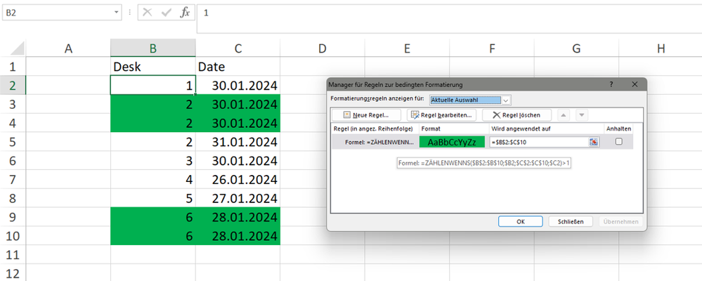
=COUNTIFS($B$2:$B$10,$B2,$C$2:$C$10,$C2)>1

You can apply this rule for conditional formatting of the sample data.

=$B$2:$C$10

This is the range the format applies to in the example.

[#3 · Accepted solution]

@Sam1209 

Let's say the desk numbers are in A2 and down, and the dates in D2 and down.

Select the rows that you want to format from row 2 down.

The active cell should be in row 2.

On the Home tab of the ribbon, click Conditional Formatting > New Rule...
Select 'Use a formula to determine which cells to format'.
Enter the formula

=COUNTIFS($A$2:$A$10000, $A2, $D$2:$D$10000, $D2)>1

Click Format...
Activate the Fill tab.
Select a highlight color.
Click OK, then click OK again.