Conditional Formatting of Rows

[Zachery David Durnell]

Hello, 

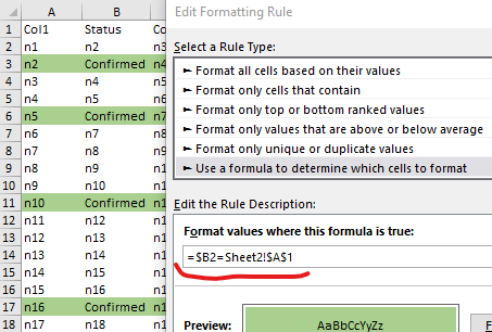
I work in recruiting and we track our interview scheduling and confirmations in excel. I have created a drop down list of statuses that we use and based off of those statuses I want the cells formatted a certain way and color. 

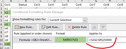
Currently, I am able to format one row or the entire worksheet, but I am not able to format multiple rows based on that status. I have attached the formulas that I am using. 

Also, please let me know if what I am asking is not clear. :) 

Thank you in advance for your assistance!!

[#2]

Hi Zachery,

I missed what is where in your sample. Assuming in column B you have statuses the rule formula could be

=$B2="Status value"

applied to your entire range. 

[#3]

Thank you Sergei. Yes, each cell in Column B has the drop down of available statuses a candidate is at in the scheduling process. 

[#4]

Hello Sergei - 

That formula did not work. I also could have been placing it in the wrong area. I have added an additional image to my clippings from that excel sheet. In theory, when both of those rows are marked as confirmed they should be colored green. The first row works fine. How am I able to duplicate that to every other row?

[#5]

Zachery, formula works if apply it correctly. Step by step

- you have data structured like this

- to color all rows with defined status the rule formula is

and the rule is applied all rows in range with some gap

Same is in attached file