Turn on suggestions
Auto-suggest helps you quickly narrow down your search results by suggesting possible matches as you type.
- Home
- Microsoft 365
- Excel
- Conditional Formatting Help Please!
Conditional Formatting Help Please!
Discussion Options
- Subscribe to RSS Feed
- Mark Discussion as New
- Mark Discussion as Read
- Pin this Discussion for Current User
- Bookmark
- Subscribe
- Printer Friendly Page
- Mark as New
- Bookmark
- Subscribe
- Mute
- Subscribe to RSS Feed
- Permalink
- Report Inappropriate Content
Mar 18 2024 07:53 AM
Hello All,
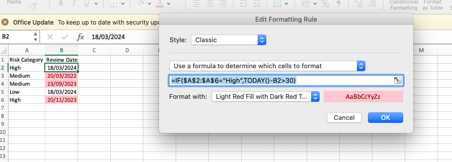
I'm trying to set up my conditional formatting so the contents of column A decide how often it needs to be reviewed.
For example, if a cell in column A is "high"I want the cell in B to highlight if the date is over 30 days old.
Then will be doing a different amount for medium and low.
This is how I currently have the formula which isn't working. It is highlighting all the cells in B that are over 30 days. I assume as the top cell is "high"
Any assistance with this would be greatly appreciated. Thanks in advance!
Labels:
- Labels:
-
Excel
1 Reply
- Mark as New
- Bookmark
- Subscribe
- Mute
- Subscribe to RSS Feed
- Permalink
- Report Inappropriate Content
Mar 18 2024 08:02 AM
