Combining 2 rows into 1 row and deleting a 3rd row

[DIverkeith]

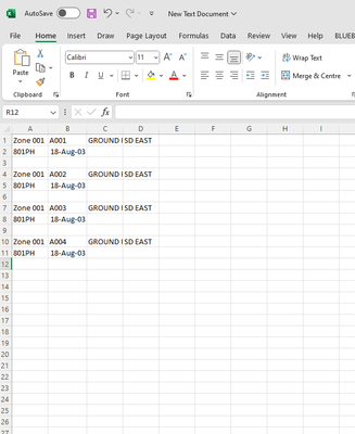
What I am looking to achieve is to join row 2 onto the end of row 1 and delete row 3, then duplicate this through the worksheet.

The data format does not change throughout 

Any ideas on the best way to resolve this into  this desired view 

[#2]

Is this a one-off or do you have to do this on a regular basis? Can you perhaps provide an Excel file with some dummy data, but in the current format?

[#3]

Does this do what you want?

=LET(c, TOCOL(A1:D1000), f, FILTER(c, c<>0), WRAPROWS(f, 6))

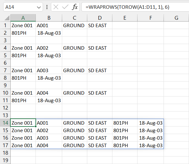
[#4 · Accepted solution]

@DIverkeith If the number of fields to be returned for each output row is always six (6) you can simply use WRAPROWS/TOROW as follows:

=WRAPROWS(TOROW(A1:D11, 1), 6)

Setting the [ignore] parameter to 1 for TOROW will ignore the blank cells automatically.

WRAPROWS/TOROW Results

[#5]

Thank you ...... That works perfectly!

Curiously how does the formulae work ... if you don't mind explaining that is 

Regards

Keith

[#6]

Thank you, this returns what I am trying to do.

[#7]

@DIverkeith No worries. The TOROW function transforms or sends the range A1:D11 to a single row, reading left-to-right, top-to-bottom by default. To see what the result of TOROW looks like, try it on its own without setting any additional parameters: =TOROW(A1:D11). Then try it with the optional [ignore] parameter set to 1 - Ignore blanks: =TOROW(A1:D11, 1). Notice how all of the blank cells are removed from the results with the second formula.

The WRAPROWS function then takes the results of TOROW (a one-dimensional array) and converts it to a two-dimensional array by "wrapping" the values into separate rows. The length of each row is determined by the wrap_count parameter, which in this case is 6.

Hopefully that helps clarify things. If you would like to read up further, exceljet does a good job of explaining both functions with additional examples:

TOROW: https://exceljet.net/functions/torow-function 

WRAPROWS: https://exceljet.net/functions/wraprows-function 

[#8]

Thank you for the explanation, Understanding how it works makes it more useable.

appreciate your time and advice