Aging Count count

[Kuppanagari_Pavani]

Hi 

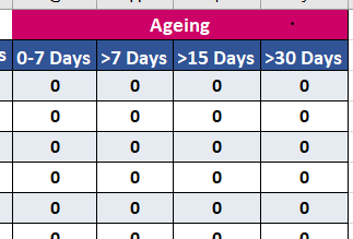
 Any one suggest As per ticket type and Priority wise and Aging bucket wise formula require for count. COuld you please help 

[#2]

Can you please explain what exactly you want or DM for further assistance. @Kuppanagari_Pavani 

[#3]

• @Kuppanagari_Pavani 

Sure, I can help you with the formula to count tickets based on ticket type, priority, and aging bucket. Here's the formula assuming your data is in the following layout:

• Column A: Ticket Type
• Column B: Priority
• Column C: Age (in days)

Excel

=SUMPRODUCT((A2:A$10=A2)*(B2:B$10=B2)*(C2:C$10>=C$2)*(C2:C$10<C$3))

Explanation:

1. SUMPRODUCT: This function multiplies corresponding elements in multiple arrays and returns the sum of those products.
2. A2:A$10=A2: This compares the values in column A from row 2 to 10 with the value in cell A2. It returns an array of TRUE and FALSE values.
3. B2:B$10=B2: Similar to the previous step, this compares the values in column B with the value in cell B2.
4. C2:C$10>=C$2: This compares the values in column C with the value in cell C2 (assuming this is the lower bound of the first aging bucket). It returns an array of TRUE and FALSE values.
5. C2:C$10<C$3: This compares the values in column C with the value in cell C3 (assuming this is the upper bound of the first aging bucket). It returns an array of TRUE and FALSE values.
6. *: The multiplication operator applies element-wise multiplication between the arrays.
7. SUMPRODUCT: Finally, SUMPRODUCT sums the products of the corresponding elements in the arrays, resulting in the count of tickets that meet the specified criteria.

Adjusting the Formula:

• Replace A2:A$10, B2:B$10, and C2:C$10 with the actual ranges of your data.
• Modify C$2 and C$3 to represent the lower and upper bounds of your desired aging buckets. You can add more comparisons within the SUMPRODUCT function to create additional aging buckets.

Example:

Assuming you have the following data:

Ticket Type Priority Age

Support	High	5
Feature	Low	12
Support	Medium	20

If you want to count tickets with priority "High" and age between 5 and 15 days, the formula would be:

Excel

=SUMPRODUCT((A2:A$3="Support")*(B2:B$3="High")*(C2:C$3>=5)*(C2:C$3<15))

This formula would return 1, indicating one ticket meets the criteria.

Remember to adapt the formula based on your specific data and desired criteria