SUMIFS with OR

[MarcoTorinoi]

I have this list:

Column A      Column B

Austria            10

France             20

Italy                 30

China               10

USA                 40

I want to sum up all the cells  in Column B if in Column A there is a European Country

=SUM(SUMIF(A:A,{"Austria","France","Italy"},B:B))

The result is correctly: 60

Now, however, the list of the European countries is much longer and I do not want to include all of them in the Array, but I want to refer to other cells where I have the list of all European countries. 

Is there a way to do it? I think in the Array it is not possible to put a reference to a cell range.

Thanks!!!

Marco

[#2]

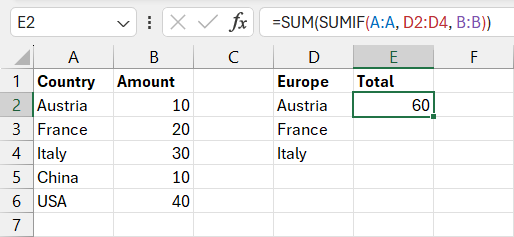
@MarcoTorinoi Don't use the curly brackets at all... just reference the range containing the list of European countries. For example, if Austria, France and Italy were listed in range D2:D4, the formula would be:

=SUM(SUMIF(A:A, D2:D4, B:B))

Note: with older versions of Excel, you may need to press Ctrl+Shift+Enter when inputting this formula.

Results

[#3]

@djclements 

Pretty strange... I get a differnt result

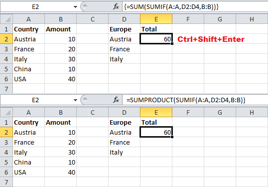
[#4 · Accepted solution]

@MarcoTorinoi Did you see my note about pressing Ctrl+Shift+Enter? If you're not using Excel 2021, Excel for MS365 or Excel for the Web, you'll need to press Ctrl+Shift+Enter when inputting that formula. Alternatively, you can also swap out SUM with SUMPRODUCT without the need for CSE:

=SUMPRODUCT(SUMIF(A:A, D2:D4, B:B))

Here's a couple of screenshots using Excel 2010. Note: the curly brackets are added automatically after pressing Ctrl+Shift+Enter (do NOT type them manually)...

Results (Excel 2010)

[#5]

@MarcoTorinoi 

Check out this formula:

=SUM(FILTER(B2:B6,ISNUMBER(FIND(A2:A6,TEXTJOIN(",",,D2:D4)))))

[#6]

Thanks. the solution with SUMPRODUCT works , ...but since I use the formula more then once in the same worksheet, the calculation is super slow and it freeze the screen for 10 or more seconds for every refresh... 😞

[#7]

@MarcoTorinoi The performance issues are caused by referencing entire worksheet columns (A:A & B:B), which means SUMIF has to process 1,048,576 rows of data for every use of this formula. Try reducing the range according to the size of your dataset (ie: A1:A1000 & B1:B1000) or format your dataset as a structured Excel table (on the ribbon, go to Insert > Table). When referencing an Excel table, the formula would look something like this:

=SUMPRODUCT(SUMIF(Table1[Country], D2:D4, Table1[Amount]))

The built-in column names of an Excel table are dynamic and will expand automatically as the table expands.

Excel Table Column References