excel in windows 10.

[Bazz02]

how to create a button that sorts by one column and then assigns an order in another column from one to 20.

[#2 · Accepted solution]

Hi, What do you mean by 'order from 1 to 20'? What is 1, what is 30? Kind regards Hans

[#3]

@hansleroy 

if you have 20 rows that have been sorted say by their %

then in another column you need show the ranking/position from 1-20

which would be 1-20 if all % were different but if for some reason some are the same 

ie the top 3, then their ranking would be 1 but the next position would be 4th and so on to the bottom if that makes sense. 

[#4]

@Bazz02 Depending on your needs and below assuming Excel 365, it can be done in multiple ways and without a macro-button.

Having data in a (pyamas) table you can calculate the rank using a column formula
=XMATCH([@Value];SORT([Value]))
...finding the value on the same row (@ = single cell intersection) among all values sorted, and returning the number of the first match.

You may sort that column using the arrow in cell C2

Since it is an interesting education example I added some more solutions outside the table;

Cell E3 sorts the table each time data changes. It is a formula in only one cell but it 'spills' the result to as many cells that are needed.

=SORT(Table1[[Text]:[Value]];2)

G3 isolates the percentages in F3:F8 by addressing E3# (includes the full spill area) and intersects it with column F using the multiple cell intersection character space.
=XMATCH(E3# F:F;E3# F:F)

If you need to redesign the layout, it may be more handy to not include a column reference and then INDEX is a solution where row number zero returns all the rows and the two tells the second col.
=XMATCH(INDEX(E3#;0;2);INDEX(E3#;0;2))

LET is yet a rather new possibility to build a complex formula step by step. Use alt+Return for line breaks.
The last row/parameter is what is shown as the output of the calculation.
=LET(range;Table1[Value];
data;SORT(range);
output;XMATCH(data;data);
output
)

[#5]

Hi,

Did you try the RANK function?

https://support.microsoft.com/en-us/office/rank-function-6a2fc49d-1831-4a03-9d8c-c279cf99f723

Kind regards

Hans

[#6]

@Bazz02 

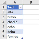
Following up some of the ideas already presented,

is returned by the formula

= LET(
    ranking, RANK(Table1[Value],Table1[Value],-1),
    output,  IF({0,1}, Table1[Text], ranking),
    SORT(output)
  )

The ranking is placed first because, for some mysterious reason, RANK requires range references and not arrays.  The next row is a device to combine the newly calculated rankings with the text column before it is sorted by rank.  

[#7]

I see that absolute references static arrays comes more and more handy. 

Using CHOOSE allows to combine multiple dynamic arrays.

=SORT(CHOOSE({3\1\2}; Table1[Text]; Table1[Value]; Table1[Rank]))

Also noted that RANK is around for backwards compatibility.

[#8]

Agreed

[#9]

All fixed , thank you

@hansleroy 

[#10]

I like Tables because of the way in which they adjust to the actual data (as well as providing structured references) so that Excel is not left to infer what is intended by the user; it is explicit.

[#11]

@PeterBartholomew1 

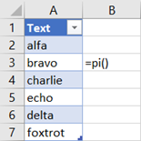
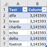
[x] Like Tables
I do though stress, during classes, that when you work with column formulas you enter it...

...and in one step gets the formula, a new column and the column filled with that formula.

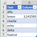
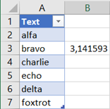
When undoing though, it demands three Ctrl+Z. One for each step.

The risk is when making a less visible change and typing Ctrl+Z, it is very easy to not have undone the change as expected. In the rest of the envirnment it is normally one change and one undo.
The only hint is a tiny green corner telling that the cell deviates.

I don't have any other suggestion for the interface - I'm confident that Microsoft have come up with the best solution among alternatives. Just notice that it is an area with a risk for unwanted results.

[#12]

@bosinander 

It can be something of a pitfall.  As a 365 dynamic array user, I tend to expect consistency and follow Ray Panko (EuSpRIG papers) in treating any individually edited term as a Latent Error (i.e. one that may deliver the correct numbers now but with no assurance that it will continue to do so during the life of the spreadsheet).  I would prefer that all edits should propagate and there should be no option to change a single term, but that would cause howls of protest.  

It is not as if any other aspect of traditional spreadsheet development makes an attempt to be robust to change, so the Microsoft default is probably a good solution, though you are correct to warn against the risk. 

Working my way, I would have

= IF([@precision]="high", 
     PI(), 
     355/113)

which, I agree, is somewhat cumbersome.

[#13]

@bosinander 

IMHO, that's always the risk to use the tool by the way it's not designed for. Structured table assumes same formula for entire column and keeps it as default formula for the column in background. 

[#14]

Definately prefer structured tables 🙂
When it comes to calculated columns it may be a safer approach to simply delete the column and make a new one. Ctrl+Space and Ctrl+- (minus) and possibly Ctrl++ comes handy.

[#15]

Microsoft has surely thought about it, but it would be appreciated by some of us to have a setting for calculated columns like
[x] All edits propagate