- Subscribe to RSS Feed
- Mark Discussion as New
- Mark Discussion as Read
- Pin this Discussion for Current User
- Bookmark
- Subscribe
- Printer Friendly Page
- Mark as New
- Bookmark
- Subscribe
- Mute
- Subscribe to RSS Feed
- Permalink
- Report Inappropriate Content
Nov 12 2023 12:42 PM
I would like to create this custom formula to calculate a points awarding system that automatically calculates. P and A are the variables in the formula.
Is this possible?
P = event finishing position
A = event attendance
Φ = fleet factor (B Fleet - 0.33; C Fleet - 0.15)
- Labels:
-
Formulas and Functions
- Mark as New
- Bookmark
- Subscribe
- Mute
- Subscribe to RSS Feed
- Permalink
- Report Inappropriate Content
Nov 14 2023 12:20 AM
What is f(x)? There is no x in the expression on the right.
And why do you sum from x = 1 to 5?
- Mark as New
- Bookmark
- Subscribe
- Mute
- Subscribe to RSS Feed
- Permalink
- Report Inappropriate Content
Nov 22 2023 05:18 PM
Yeah, I was not much at math... so alot of the characters don't mean much to me... however...
The formula creates a point system for overall points for a sailboat racing season. The points awarded are dependent on the number of entries in the race, and the position of each boat in that race.
there is a graph that has the detail but I am trying to put the formula into excel for easier calculation...
if it works that is....
does that help?
- Mark as New
- Bookmark
- Subscribe
- Mute
- Subscribe to RSS Feed
- Permalink
- Report Inappropriate Content
Nov 22 2023 06:32 PM
or constant?
I guess need some specific variables and expected result to understand this formula.
- Mark as New
- Bookmark
- Subscribe
- Mute
- Subscribe to RSS Feed
- Permalink
- Report Inappropriate Content
Nov 22 2023 08:22 PM - edited Nov 22 2023 11:23 PM
@pevenden If you have Excel for MS365, you can achieve the same results as the graph you've shared with the following formula:
=LET(n, B1, k, B2,
φ, IF(ISBLANK(k), 1, k),
MAKEARRAY(n, n, LAMBDA(p,a,
   IF(p>a, "", IFERROR((p*(1-((50*a+4800)/98))+((a*(50*a+4800))/98)-1)/(a-1), 25)*φ))))
...where the attendance (A) is in cell B1 and the fleet factor (φ) is in cell B2. The results would look something like this:

Conditional Formatting was applied to range C5:V24 to shade the empty string results blue using the following formula:
=AND(NOT(ISBLANK(C5)), C5="")
You could also create a custom LAMBDA function in Name Manager to award points to each team based on their finishing position for each race. For example, you could create a function called XPOINTS using the following formula:
=LAMBDA(a,p,[φ],
   LET(
      k, IF(ISBLANK(φ), 1, φ),
      IFERROR((p*(1-((50*a+4800)/98))+((a*(50*a+4800))/98)-1)/(a-1), 25)*k
   )
)
...then use it as follows:

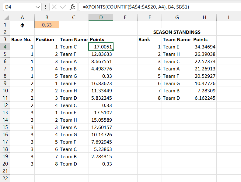
The formula used in cell D4 in the screenshot above is:
=XPOINTS(COUNTIF($A$4:$A$20, A4), B4, $B$1)
...where COUNTIF is used to calculate the total attendance (A) for each Race No.
As for the Season Standings section shown above, the following formula was used in cell F4:
=LET(
u, UNIQUE(C4:C20),
a, SORT(HSTACK(u, SUMIFS(D4:D20, C4:C20, u)), 2, -1),
HSTACK(SEQUENCE(ROWS(u)), a))
I've also attached the workbook for your convenience. Cheers!
- Mark as New
- Bookmark
- Subscribe
- Mute
- Subscribe to RSS Feed
- Permalink
- Report Inappropriate Content
Nov 22 2023 08:25 PM - edited Nov 23 2023 07:50 AM
If you google "event finishing position" "event attendance" "fleet factor" with quotes, we find the HCA Competitive Ranking formula (click here).
The formula (from page 1) is not proper math. It might be parsed as follows:
The formula f(x) calculates the points assigned to a participant based on the participant's position (P = 1 to A) in a race with "A" participants.
The notation Sigma(f(x), for x=1 to 5) simply means: sum the points from 5 races.
In particular: ``the system includes your best five regatta finishes. If you sail fifteen events, we take your very best results for your ranking``.
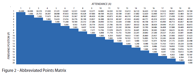
The table below (from page 2) shows the expected f(x) before applying fleet factor (phi) for finishing positions (P) in races that have A=1 to 20 participants. It is just an example.
Note: I don't know if it is implicitly suggesting that f(x) should be rounded to 3 decimal places. Further reading might be necessary.
"The remainder of the solution is left as an excercise for the student". (wink)
- Mark as New
- Bookmark
- Subscribe
- Mute
- Subscribe to RSS Feed
- Permalink
- Report Inappropriate Content
Nov 22 2023 08:59 PM
@pevenden as per the new information provided by @JoeUser2004 regarding "the system includes your best five regatta finishes", the formula to generate Season Standings in my above response can be modified to sum the results of each team's best 5 finishes as follows:
=LET(
u, UNIQUE(C4:C20),
a, BYROW(u, LAMBDA(r, SUM(TAKE(SORT(FILTER(D4:D20, C4:C20=r)), -5)))),
HSTACK(SEQUENCE(ROWS(u)), SORT(HSTACK(u, a), 2, -1)))
Please see the attached updated workbook (v2).
- Mark as New
- Bookmark
- Subscribe
- Mute
- Subscribe to RSS Feed
- Permalink
- Report Inappropriate Content
Nov 23 2023 09:37 AM
I have Office Professional Plus 2019
! am not worried about the 'top 5 finishes', I am using this for a different sport 'Horse competition' where each 'class' can have anywhere from 3 to 15 riders.
the 'class' competes 6-8 times per season, and the number of riders vary each time. The season points will include all events. Also, I am not worried about a 'fleet factor'
@djclements if I alter B2 to a different number instead of 20, say 10, all i get is this: #NAME? in all the cells...
- Mark as New
- Bookmark
- Subscribe
- Mute
- Subscribe to RSS Feed
- Permalink
- Report Inappropriate Content
Nov 23 2023 03:48 PM
@pevenden No worries. The functions I used in the those files will only work with MS365. The main formula that can still be used in Office 2019 for calculating points is:
=(p*(1-((50*a+4800)/98))+((a*(50*a+4800))/98)-1)/(a-1)
...where p is the Position, a is the Attendance, and the Fleet Factor has been omitted.
I've attached another workbook (v3) that should work with Office 2019. In this version, I used Excel Table formatting, with calculated columns for Attendance and Points. The formula used to calculate Attendance is:
=COUNTIF([Race No.], [@[Race No.]])
And the formula used to calculate Points is:
=([@Position]*(1-((50*[@Attendance]+4800)/98))+(([@Attendance]*(50*[@Attendance]+4800))/98)-1)/([@Attendance]-1)
Note: I've excluded the IFERROR function here, as you have stated the minimum number of riders in any given race is 3, so the above formula will return the #DIV/0! error when only 1 rider has been entered in the table for a given race.
Add new data to the bottom of the table by inputting values in the Row No., Position and Jockey columns. Data Validation was used in the Jockey column to select from a list. The source for the pick-list is the Jockey column from the Season Standings table.. adding new Jockey names to this table will make them appear in the pick-list.
After inputting new data, sort the Season Standings table by the Total Points column from largest to smallest to refresh the standings.

- Mark as New
- Bookmark
- Subscribe
- Mute
- Subscribe to RSS Feed
- Permalink
- Report Inappropriate Content
Nov 23 2023 05:16 PM
I will play with a bit (I've created a new 'test' sheet so I don't mess up your formulas... )
and I think it will do the job perfectly...
thanks everyone for your help in sorting this out...


