Can you use AND / OR in an INDEX MATCH

[David]

Hi I have am array formula that looks like this:

=INDEX('Rebate report'!A:A,MATCH(1,('Rebate report'!A:A=A2)*('Rebate report'!B:B=B2)*('Rebate report'!C:C=C2),0),1) which works.

I want to add in an OR function for the name in column A. I will add this name in Column T. In other words the match is correct if column A or T match A2 and COL B=B2 and COL C=C2 also match the criteria

I tried using the + to add T criteria but gave me a 0

=INDEX('Rebate report'!A:A,MATCH(1,('Rebate report'!A:A=A2)*('Rebate report'!B:B=B2)*('Rebate report'!C:C=C2)+('Rebate report'!A:A=T2),0),1)

Thanks for the help!

[#2]

@RODRI1611 , you are welcome

[#3]

Hi,

Is it possible to look for one of two things in a column?

Eg, I want to search for apples OR bananas In the list:

Apples - £1.50
Oranges - £0.50
Pears - £3.20
Berries - £3.30

How is this done?

Thank you

[#4]

Sorry my above question was meant for you Sergei

[#5]

@Buzztank 

Couple of variants are in attached file

[#6]

Hi @Sergei Baklan 

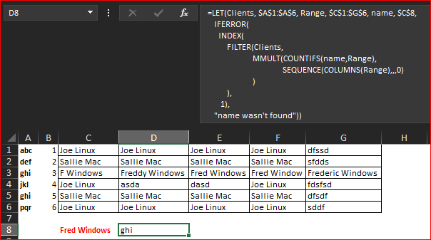
I am looking for something very similar to the formula you created for Johnny but I'm having no luck googling a solution. You mentioned the formula only works is the values in each column are never the same. But is there any way to modify the formulas so that it would work if some values were the same?

The reason I ask is that I have a workbook that compiles client data from across 5 different databases. A mini master data table. Each row = 1 client. And for each client in the table there's 5 client name columns (1 name from each database). Sometimes they're the same but often there's discrepancies between the 5 DBs.

So I'm hoping to write a formula that says if you match "Freds Windows" in any of the name columns say C:G then return the account reference number in column A:A

Is something like that possible?

All the best

Vicky

[#7]

@Vicky1234 

If I may offer a suggestion, I believe what you want to do will be the same except you just need to test if the sum of the OR conditions is> 0. So,

((C:C="Fred Windows)+(D:D="Fred Windows)+(E:E="Fred Windows)+(F:F="Fred Windows)+(G:G="Fred Windows)>0)

Of course, the above conditional test would then be multiplied by any AND conditions you have.

See attached for some examples. Note that if you don't have office 365 with dynamic arrays, then you will need to hit Ctrl+Shift+Enter after keying the formula instead of just enter.

[#8]

@Vicky1234 

Here is practically the same idea as @JMB17  suggested but for Excel 365, plus I understood the logic of source data in a bit different way

with

=LET(Clients, $A$1:$A$6, Range, $C$1:$G$6, name, $C$8,
   IFERROR(
     INDEX(
         FILTER(Clients,
                MMULT(COUNTIFS(name,Range),
                      SEQUENCE(COLUMNS(Range),,,0)
                )
         ),
      1),
   "name wasn't found"))

[#9]

@Sergei Baklan 

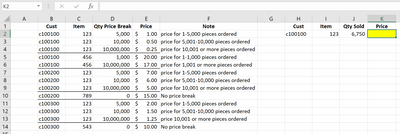
I'm trying to create a formula that will bring back the price for a specific customer and item combination. The part I'm having issues with is with the quantity sold. Some items have a singular price (meaning if the customer buys 1 piece or 1,000 pieces, they are going to pay the same price), while other items have price breaks depending on the quantity they buy. For example, if the customer buys 1-500 pieces of item 123, they'll pay $1. If they buy 501-1,000 pieces of item 123, they will pay $0.50.  Any advise would be appreciated!

[#10]

@Sergei Baklan 

Hi Sergei, 

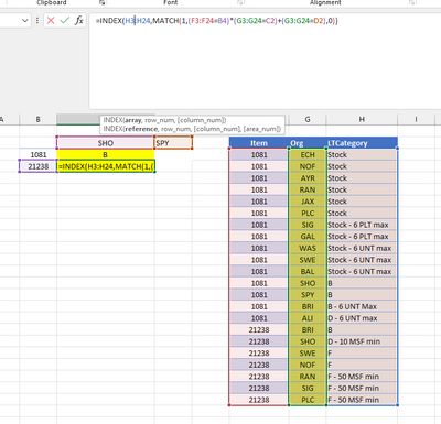
I'm trying to do something similar but running into an issue where an incorrect value is returned when I drag down the formula to other item numbers, 

I need to find column C where column A=A2 and column B = SPY or SHO

Item	Org	LTCategory
1081	ECH	Stock
1081	NOF	Stock
1081	AYR	Stock
1081	RAN	Stock
1081	JAX	Stock
1081	PLC	Stock
1081	SIG	Stock - 6 PLT max
1081	GAL	Stock - 6 PLT max
1081	WAS	Stock - 6 UNT max
1081	SWE	Stock - 6 UNT max
1081	BAL	Stock - 6 UNT max
1081	SHO	B
1081	SPY	B
1081	BRI	B - 6 UNT Max
1081	ALI	D - 6 UNT max
21238	BRI	B
21238	SHO	D - 10 MSF min
21238	SWE	F
21238	NOF	F
21238	RAN	F - 50 MSF min
21238	SIG	F - 50 MSF min
21238	PLC	F - 50 MSF min

[#11]

@mquigley 

[#12]

@mquigley 

Please use absolute references in formula for all except B2

H2:H24 => $H$2:$H$24 etc

Switch between relative, absolute, and mixed references (microsoft.com)

[#13]

@Sergei Baklan 

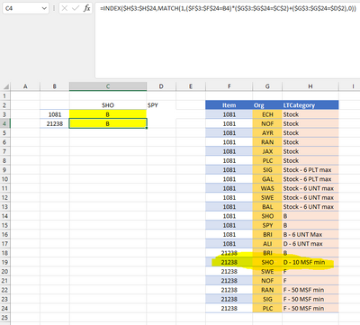
Thanks for your help! For some reason I'm still not seeing correct values after updating the absolute references and hitting Control Shift Enter. The correct return value in C4 should be H19.

[#14]

@mquigley 

Missed that, sorry. MATCH shall be as

, MATCH( 1, ($F3$F24=B4)*( ($G3$G24 = $C$2) + ($G3$G24 = $D$2) ), 0 )

* works as AND and + as OR

[#15]

Thanks so much, that worked!

[#16]

@mquigley , you are welcome

[#17]

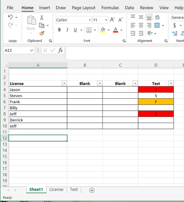
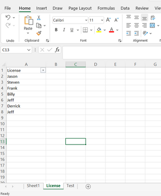
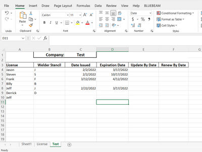
@Sergei Baklan Can you assist with a formula.  I have three sheets: Sheet 1 which is my main screen, License, which is a list of my employees, and Test which is one of my required certifications.  Sheet 1 column A automatically pulls from License for my employee names.  i would like for Column "D" of sheet one to pull the value of column "B" of test if there is a value in column "C" of Test and if Column "A" of Sheet 1 matches Column "A" of Test.  

ive used an index and match statement but when i filter the values are not correct.  

[#18]

@sannese 

In D4:

=IFERROR(LET(n,MATCH(A4,Test!$A:$A,0),IF(INDEX(Test!$C:$C,n)>0,INDEX(Test!$B:$B,n),"")),"")

Fill down.

[#19]

@Hans Vogelaar thank you very much.  i think i can make that work. 

[#20]

@Hans Vogelaar, i have a follow up question to your prior response. I am trying to work with conditional formatting to highlight "Sheet1" Column "D" red when the date of "Test" Column "D" is within 30 days of the current date for the matching name in Column "A". i can get it to work but when i sort by "Sheet1 Column "A" the conditional formatting does not sort.

[#21]

@sannese 

Select D4:D10 (or however far down the data go) on Sheet1.

D4 should be the active cell in the selection.

On the Home tab of the ribbon, click Conditional Formatting > New Rule...

Select 'Use a formula to determine which cells to format'.

Enter the formula

=VLOOKUP($A4,Test!$A$4:$D$100,4,FALSE)<=TODAY()+30

Change 100 to a larger number if you expect to populate below row 100 on the Test sheet.

Click Format...

Activate the Fill tab.

Select red.

Click OK, then click OK again.

The conditional formatting should now move with the cells if you sort the range.