Can I make a cell value appear only after a certain date?

[Sam Maw]

Hello, I'm a beginner here. Is there a formula or function I can use (perhaps a =IF?) where I can make a certain formula's value appear in a cell only after a certain date? 

Context: on each month's sheet of my annual budget spreadsheet, I have a cell showing me that month's income minus expenses.  On a separate summary sheet for the whole year, I would like to see that value for the month only after the month is over (ie, it only shows me June's income - expenses on or after July 1st). 

Hope that makes sense. Thanks. 

[#2]

I manually add and subtract them from the table when they join/quit.

[#3]

@mstingle 

Afraid that doesn't work, that's only if copy the formulas with calculations for previous period and paste the as values, after that add to totals.

I'd add to the column one more column where you may put any character if member quit and make calculations taking it into account. To show only active members you may filter the table by that column.

[#4]

@Sergei Baklan is it possible for me to create a cell of text that appears after I enter a date? For example if i entered between the dates of "1965-1975" how do I make it say 'pinapple' or anything like that. I hope you understand what I'm asking? (If it is possible? How?)

[#5]

@Harry_Chubb 

Afraid not, it's better with sample file.

If you enter some text which includes dates in which exactly format you enter them (with dash, dash and spaces around, whatever).

If you enter couple of years how Excel knows this exactly range shall be marked as 'pinapple', not something else?

If ranges are overlapping?

Where to show marks?

Perhaps something else, but better illustrate on the file with manually added desired result.

[#6]

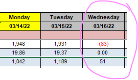
@Sergei Baklan Please can you help me with having a cell not calculate until two days after the current date?  I have to update a daily metrics sheet that contains worked hours, but our information is always two days behind.  For example, if today is Thursday, I will send out Monday's figures, (Friday's = Wednesday, but Monday, since it is two calendar days past, I can send out the full previous week, just as long as it is two calendars days past, it is okay for the formulated cell's calculation to show up).  The problem is we have managers who enter transferred hours into the previous and sometimes, current date and those show up in the Week-To-Date and Month-To-Date columns.  I do not want them to show up there until the other information is there, too.   I pasted an example.  The Wednesday information should not calculate until Friday, but it is calculating into the To-Date columns.  I have been asked to get this information out of the daily reporting, and I do not want to have to paste in the new formulas each day. :(  Please, can you help me?  Thank you.

[#7]

This discussion really helped my issue. I calculate on a specific date but once the date passes the formula wipes out my information. How do I get the formula to function on one day and retain that information once the date passes.
=IF(TODAY()=DATEVALUE("2023-02-07"),INDEX(PLAYING!$E$1:$G$200,MATCH(DE4,PLAYING!$E$1:PLAYING!$E$200,0),2))

TEAM # GROSS HDCP 14 L
ACOBA, JEFF 25 11 14 L
formula resides in cell and looks at ACOBA, JEFF and finds his handicap (11) and populates. I want this to populate on correct date but once that date passes I want the information to stay and not change. Help please.

[#8]

@James_Pape   I was able to work with a colleague and he helped me find the way.  It appears two calendar days after the date in the top of the column.  you can adjust it to not have the "+2".  It appears with the date you indicate and stays there.      

"=IF(TODAY()>=(N$2+2),VLOOKUP(N$2,'H:\"  the rest of my formula is after the H.  but the part you need is, "=IF(TODAY()>=(N$2+2),"  the N2 cell is where i have the current date, in row 2.

I hope I understood your question and this helps you.    

[#9]

@Adrienne_Ali 

Thank You for your efforts.  But, still have an issue.

I understand your "=IF(TODAY()>=(N$2+2)"

=IF(TODAY()=(DD$2+2),INDEX(PLAYING!$E$1:$G$200,MATCH(DE4,PLAYING!$E$1:PLAYING!$E$200,0),2))

This does calculate my cell two days prior to current date which I can work with, but, once the date has passed the formula returns a "false" there for removing the number that I need to stay.

I included my sheet so you can look at it.  I made my changes to Week 19, DE4 and used DD2 for date info.  

What I am looking for is for DG4 to calculate on a certain day.  Your addition calculates 2 days after date in DD2.  On third Day DG4 reverts to a "FALSE" and clears my number.  I need it to calculate on a certain day and retain that information for 18 weeks in that cell DG4.  Because the number that it is looking up can change from week to week.

So what I do now is calculate all players in column DG and then copy and paste value each week.  But I can not figure out how to keep the numbers in DG from changing once it has calculated on its correct date.

I hope this makes sense.

Thank You

James Pape

[#10]

It does makes sense, but what you need is beyond my scope of Excel. I am sorry. Perhaps someone reading these threads can chime in and help you.

[#11]

Adrienne, Thank you for your efforts. I will keep trying to find a solution. I know there has to be but so far it has escaped me.
Jim

[#12]

@James_Pape 

Try using ChatGPT to find a formula that works! 

[#13]

Hey Ashleigh143,
I am not sure what ChatGPT is. I have never done this so not sure where to start.

[#14]

Ashleigh143,
Thanks I found it and am working on its response. Thank You.

[#15]

@James_PapeAshleigh143

Well, I have a answer to my problem.  My daughter is a security engineer for a bank and I had her set down with me.  My original formula only looked at a certain page, PLAYERS!.  Well the answer was to create a different PLAYER! sheet for each week.  So, I have PLAYERS1, PLAYERS2, and so on.  These are pointed to by each week in my "MATHCH PLAY TWO" sheet. 

So my final formula for each week looks like this.  

=INDEX(PLAYING8!$E$1:$G$200,MATCH(AQ4,PLAYING8!$E$1:PLAYING8!$E$200,0),2) 

Which is week 8s column.

So, when my PLAYING sheet is updated I just copy and paste the information into the PLAYING? week that we are working on.  Cures all my issues and I am looking back and laughing at myself.

Thanks again for you help.

Jim

[#16]

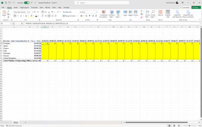
@Sergei Baklan Hi, I have seen your guidance and must appreciate your knowledge.  I have tried the same formula, where I want 1 in every cell after the chosen date and the earlier cells with dates should apprear ZERO.  The formula isn't working for some reasonFile .  Any guidance will be appreciated.  Thank you.

[#17]

@jqnkjq 

Unfortunately link on the file is wrong, it's on your local file mapped with OneDrive. To share outside open OneDrive in browser, for the file to share in 3-dot menu find share, follow instruction to generate the link (be sure file shall be available for everyone) and share the link here.

Base on screenshot. If you have actual dates both in column C and in headers, when it could be like

=IF($C7 <= D$6, 1, 0)

and drag it to the right and down.

If you have texts which looks like dates when we need to parse such texts and convert to actual dates. When we need bit more information, where are dates and where are texts.