Custom Formulas for Calculations in Pivot Table

[Gaurav Chhabra]

Hi,

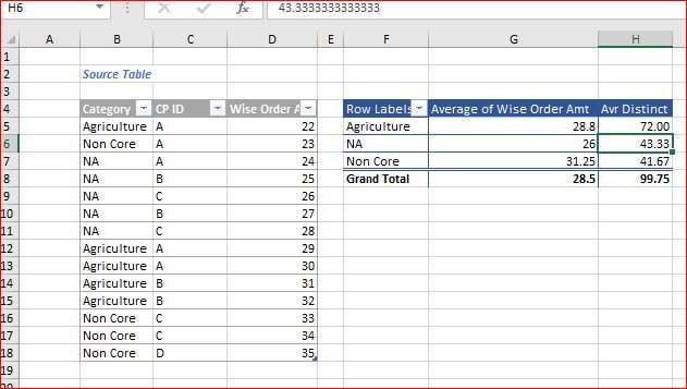
How to ADD custom formula for calculation in pivot-table. I'm using "Data Model" in the pivot, See attachment.

[#2]

Hi Gaurav,

If you add the table to data model you may use Power Pivot for further analysis. However, isn't  included into all Excel versions https://support.office.com/en-us/article/Where-is-Power-Pivot-aa64e217-4b6e-410b-8337-20b87e1c2a4b?u...

If you don't add to data model you may add calculated fields using Analyse->Fields,.. menu in Ribbon for PivotTable tools (whenyou stay within it).

[#3]

Hi Sergei,

I've my sales of last year, Two major heads in it is "Sales executive" and "Category"
I need to show the average sales by "Sales Executives" in particular category.

I'm using average function but it devide (Total Sale/Count Sales Executive) instead of (Total Sales/ Uniwue Count Sales Executive).

As sales sheet includes multiple row for each sales executive, this is the main issue.

[#4]

Hi Gaurav,

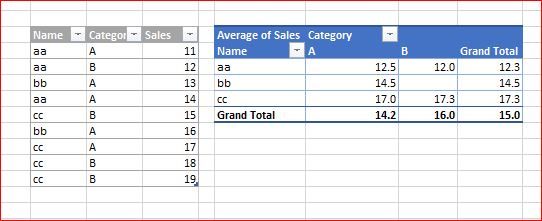
Sorry, i din't catch - if you use Pivot Table why do you need any additional function for that? That could be like this

If something else need bit more details.

Just in case, how to claculate distinct count (outside the data model and pivot tables) is here https://exceljet.net/formula/count-unique-text-values-in-a-range

[#5]

How about:

- right click on the values within the PivotTable

- summarize as ... --> average

Best, Oliver

[#6]

Hi Sergei,

Appreciating your help!

Hope in this attachment I'm delivering the proper information to you what I need.

I need this manual calculation to be done in pivot as I'll link a graph so the calculation should vary as per changes in the pivot.

[#7]

Hi Oliver,

Appreciating your help!

I need this manual calculation to be done in pivot as I'll link a graph so the calculation should vary as per changes in the pivot.

[#8]

Hi Guarav,

Okay, i see. When one more to clarify - it looks like using of data model is not the mandatory option for you, correct? 

[#9]

Hi Sergei,

No, its not necessary!, I used it just coz it allows me to show the "Distinct Count", which i thought to use in measuring required average sales, but now in data model option its custom formula option is disabled.

[#10 · Accepted solution]

Hi Gaurav,

As usual there are few ways to do that, depends which version of Excel do you have and how you are familiar with data model aggregations.

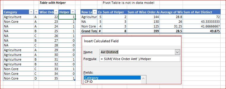
1) That's without using data model

- Add to your table helper column to calculate distinct number like

=IF(SUMPRODUCT(($F$5:$F5=F5)*($G$5:$G5=G5))>1,0,1)

- Create Pivot Table WITHOUT adding it to data model

- From Analysis menu add calculated field to average based on distinct count

=SUM(Wise Order Amt)/Helper

2) If your version of Excel is with Power Pivot you may

- from Power Pivot menu add your source table to data model

- within Power Pivot add measure as

Avr Distinct:=SUM(SourceTable[Wise Order Amt]/DISTINCTCOUNT(SourceTable[CP ID])

- from Power Pivot add to excel PivotTable with updated bu above measure data model

3) If you don't have Power Pivot.

You don't have direct access to data model from within Excel (I still can't understand why Power Query is free for everyone with any Excel, and Power Pivot is only for "Pro" versions. But that's another story).

However, there is the workaround.

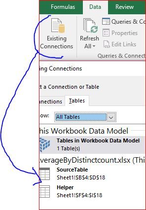
- Based on your source table add any tiny Pivot Table with ADD TO DATA MODEL option. At any place and with any one field - after that you don't need it any more. The only purpose of this pivot table is to add your source table to data model

- Find in menu Data->Existing connections, select here your source table and add it to Excel as new table

- you shall receive exact copy of your source table

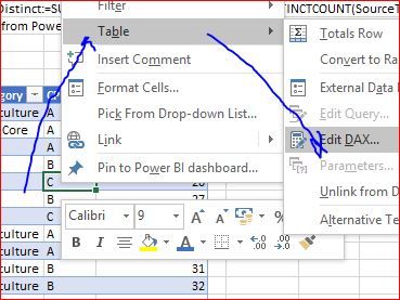
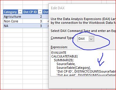
- to check, right click within the table as on screenshot and find edit DAX

- now a bit of DAX coding is required. That's not a rocket science, based on sample below and with some help from Google i believe you may modify the sample for your needs

EVALUATE
CALCULATETABLE(
   SUMMARIZE(
      SourceTable,
      SourceTable[Category],
      "Dst CP ID", DISTINCTCOUNT(SourceTable[CP ID]),
      "Dst Avr Amt", DIVIDE(SUM(SourceTable[Wise Order Amt]),DISTINCTCOUNT(SourceTable[CP ID]))
   )
)

Here

EVALUATE returns expression after it to Excel as the table

SUMMARIZE is the builder of the table,

First parameter is the name of your source table as it is in yout Excel sheet  (in my case i simply called it SourceTable),

After that separated by comma fields you'd like to add to your new table. If you repeat the name of your source table thats simply TableName[Field Name] (e.g. SourceTable[CP ID]).

If that will be calculated field you first shall add string with such field name and after that the expression with its calculation.

I guess names of aggregation functions in the sample are self-explained.

- Copy you DAX code and add to new table through Edit DAX right click menu

- now you have the table with desired fields (it's refrshed by right click menu or by Data->Refresh All). You may build your chart directly on this table, or based on this new table create one more PivotTable. (to add slicers, etc)

File with sample is attached

[#11]

Hi Gaurav,

Sorry, forgot about much more straigtforward way. Working on daily basis with Power Pivot don't remember all workarounds.

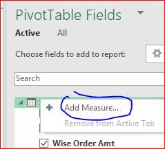
So, create your PivotTable adding it to data model. When right click on table name and select Add measure

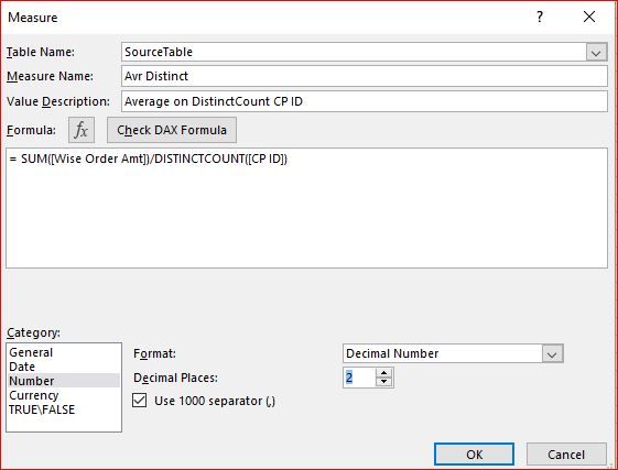
and define your measure in next window like

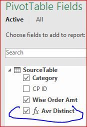
New field appears for PivotTable which you may add to you table

[#12]

Hello Sergei,

Thanks!

It's done! :)