formula help
17 Topics
Outlook template with date
Hi everyone, I'm trying to set up an Outlook template that includes an automatic date (prior date from today) within the text. For example instead of saying ''Please find attached the report from last Saturday'' It would calculate automatically what was the last saturday from today's date ''Please find attached the report from Saturday [x]'' I found that in your template you can 1. Insert/ Date and time/ Update automatically 2. Right click on your date/ Toggle Field Codes That way it displays the {DATE} field. It gives you the option to change the formatting beyond the limited choices in the dialog box. But I can't figure the formula from there... Any Idea how ? and what would be the formula ? Any Alternative ?4.4KViews0likes0Comments
Formula help needed
Hi all. I need help with a simple formula, I've been trying for days, but I'm unable to find a solution... In a list, I have: A column called [Power] with choices from 1 to 4. A column called [Impact] with choices from 1 to 4. A column called [Total_Score] with formula= [Power]*[Impact]. My quest: A column called [Management_Style], a calculated column, where I would like to make a matrix (powerXImpact) Matrix: If power =3 or 4, and impact = 3 or 4; then "Manage Closely" If power= 3 or 4, and impact =1 or 2; then "Keep Satisfied" if power = 1 or 2, and Impact = 3 or 4; then "Keep Informed" If power= 1 or 2, and impact= 1 or 2; then "Monitor (Minimum Effort)" I tried many types if multiple IFs, ANDs, ORs, but I could not find the right formula. Any help is really appreciated. Thank you all!Solved1.2KViews0likes1CommentUsing calculated formulas for time in lists
I have [Check-In] and [Check-Out] time and date column entries I then have a [Total Time] calculated column which uses this formula =TEXT([Check-In]-[Check-Out],"h:mm") I can get the total time, however I need to be able to set an IF for if the [Lunch Break] column yes/no is "Yes" it will deduct -0.5 or 30mins in the [Total Time] I have attempted a few methods however I keep getting syntax or incorrect values.Solved8.3KViews0likes2CommentsFormulas to highlight cells
Hello! Thank you so much in advance for your help! I have a cell in A1 that contains: Composer A (BMI) 50% [292650159], Composer B (ASCAP) 30% [154541151], Composer C (SESAC) 10% [55547898], Composer D (SESAC) 5% [4125475], Composer E (SOCAN) 5% [02124054] 1) I'd need a formula to use in Conditional Formatting that will turn this cell green if the sum of the % equals 100%. 2) I'd need another formula to turn the cell red if the sum doesn't equal 100%, and no highlighting if the cell is empty. *** I have another cell in B1 that contains: Publisher A (BMI) 50% [612559885], Publisher B (ASCAP) 35% [02135474], Publisher C (SESAC) 15% [01023545] I'd need a formula to highlight the cell in green if the percentages for BMI and SESAC match the ones in the previous cell (A1) for composers and if the sum of all the % in this publisher cell equals 100% (SOCAN composers go under the ASCAP publisher in this example that's why there is no Publisher for SOCAN). The cell should be red if there is an issue with the % splits. I really appreciate your help! Thanks again!846Views0likes0Comments
Formula help
I am looking for some help with formulas. I am creating a QC document to check competence of Agents. The document includes an overall outcome section, plus the detail of all components. Currently I have the following formula in the document to determine the outcome of the call: =IF((OR(M14="No",M16="No",M18="No",M20="No",M22="No")),"Family at risk","Family cared for") This works on it's own but I am now trying to create an annual summary that will collate the results from multiple QC's completed. However, when the detail components are blank (not yet completed), the formula i have defaults to an outcome showing "Family Cared for". On my summary sheet however, this causes problems as it shows as this having an outcome. Is there a formula i can use for my outcome section (as shown by formula above) which when blank and uncompleted also shows as blank in the outcome box. I hope this makes sense. Thanks,723Views0likes0CommentsPayment Tracker Calculator
Hi! I am trying to create a spreadsheet in excel to subtract payments and give an ending balance, but unsure of what formula to use or how to input. I want it to be set up to automatically calculate without me having to enter the formula in each cell, but I'm unable to do so. Here's a screenshot for reference. Any assistance would be greatly appreciated.Solved2.7KViews0likes4Comments
Excel Formulas and Functions
I'm creating a spreadsheet to help keep logs of jobs I do daily and weekly. I need a formula to add rows in a column, then subtract a certain amount as long as the amount is over a certain amount.. Example; I have 4 or 5 rows that the amounts are over $51.00 I need to add those rows and then subtract $14.00 from each unless the amount is under $51.00 then I need to subtract $6.002.9KViews0likes6Comments
Help with Completed Date Formatting in Calculated Column
In search of a formula that will calculate the working hours Monday-Friday , 8 hour days. Excluding weekends. The reason is, I am looking for real duration of project during working hours. Currently I have the below as the Calculated formula, but need to get the hours correct. =TEXT([Completed Date]-Created,"h:mm") Thank you!Solved1.4KViews0likes2CommentsVBA code: Count number of times a cell is changed if cell = Yes
I'm currently using a VBA code that tells me in Cell B15 the current number of times Cell C15 has changed, and that's great, but I have other cells (Cells F16 through F100) that I'd like to have start at a base of 1 and add 1 to the base value each time the specific cell changes if the other cells are activated via the keyword "Yes" in Column D (Cells D16 through D100). Not all of the cells are going to be activated at the same time and I'd like to be able to reset the number if at all possible to have it scale up more than once. Here is the formula I started with that is keeping track of the first changed cell. Private Sub Worksheet_Change(ByVal Target As Range) Dim xRg As Range, xCell As Range On Error Resume Next If Target = Range("C15") Then xCount = xCount + 1 Range("B15").Value = xCount End If Application.EnableEvents = False Set xRg = Application.Intersect(Target.Dependents, Me.Range("B9")) If Not xRg Is Nothing Then xCount = xCount + 1 Range("B14").Value = xCount End If Application.EnableEvents = True End Sub3.2KViews0likes0CommentsFormula Problem Countif based on Unique value and based on another comlum
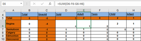
I will first off say I am a travel agent to give you some context on what I use this information for. I have basic knowledge in Excel and it has all been self taught. For this spreadsheet my Microsoft Flow will input data into this spreadsheet and the counter at the top will keep track of how many seats/rooms I have sold vs unsold for group bookings. *For the number of people I think I have it figured out. The only correction I would try and make is counting adult seats. My way works but I dont think this is the best way. Ideally I would like to count adults it counting the number of people that do not have a value in the Child's Age Column. If that cant be fixed then that's fine. What I am using right now is just Minus-ing the amount of teens/kids/infants. ds/infants Now Onto my bigger issue and the main reason why I am posting. Counting the number rooms is more difficult. Each room is generated an ID through Microsoft Forms/Flow. This is their "room number". 1. For L5 I would like it to be total of Junior Suite Rooms. From what I am thinking it has to count the unique values (room number) from a14:114 and it has to match it with what rooms (k14:k114) that are labeled as Junior suites. I believe I have use a countif or sumif but all the different ways wont work for me. This would = the amount of Junior Suites I have sold (Keep in mind I dont just want to count all the Junior Suites(K14:k114) since sometimes there is anywhere from 1-4 people in a room) 2. Now After that I want to calculate L6, L7, L8, L9,L10, etc. What I want it to do is calculate the unique values from Room Number (a14:a114)+match the rooms labeled as Junior Suites (K14:k114)+ match it with the Departure city (H14:114)(Regina, Saskatoon, etc.) This would then = the amount of Junior Suites I have sold from Regina (or Saskatoon, etc) Total Number of rooms is a number I put in (no formulas). Then once I have the above two situations figured out "unsold" as a simple formula. For example "total"-"sold"= unsold. This is something I know how to do. Thank you in advance!! Between this and Microsoft Flow this is going to save me so much time and I am super excited! Thank you, Samantha1.2KViews0likes0Comments