formulas and functions
25427 Topics
I'm looking for a practical way to calculate Pakistan salary income tax in Excel.
The goal would be to enter a monthly salary and have the spreadsheet estimate the applicable tax and resulting take-home amount. Ideally, the calculation should be easy to update when the applicable tax slabs or salary-related rules change. For someone building this in Excel, would you recommend keeping the tax slabs in a separate lookup table and using formulas against that table, rather than hard-coding the rates into one large formula? I'm particularly interested in approaches that make the spreadsheet easier to maintain when tax rules change.20Views0likes1Comment
Webservice function
Hello. I want to use the WEBSERVICE function to geolocate an IP address. The address is in cell A1, and the function is in A2. The function looks like this: =WEBSERVICE("https://ip-api.com/csv/" & A1). Unfortunately, the result is #ARG!. I have no idea what is wrong. Can you help me? Best regards, Piotr122Views0likes3Comments
Linked data not updating
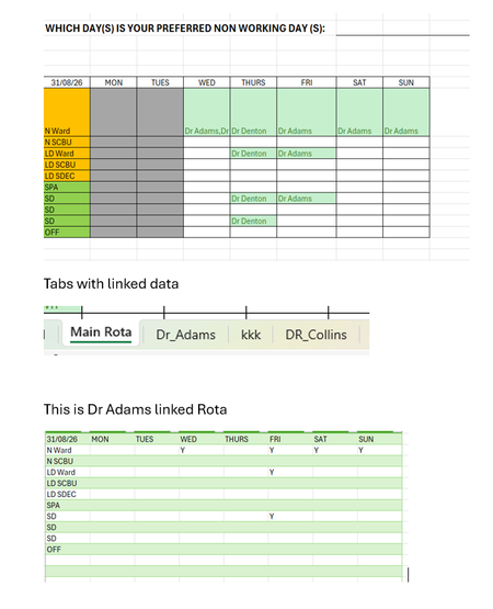
Hi I have a rostering spreadsheet where each person has their own spreadsheet with their rota they select a shift in their spreadhseet. I have a main spreadhseet where I link each spreadhseet to my my main rota so I can see what shifts they have selecteeneed and be able to resolve any conflicts i.e 2 peole selecting sam eshift. The issue is when data is updated in the individual spreadhseet it is not pulling through to my main spreadsheet. I used Data and get data form Excel file to link the workbooks. Not sure what I am doing wrong When Dr Adams adds a Y in Thursday it is not showing in my spreadhseet177Views0likes2CommentsReferenced cells do not identify themselves with color
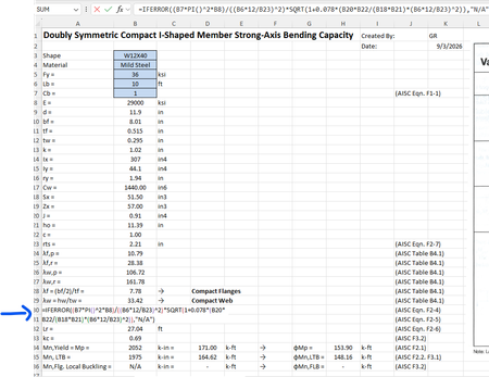
For some reason when I create a formula that references other cells, I cannot get those cells to "identify" themselves with a specific color. For example, in the image below the formula references cells B7, B8, B6, etc but they are just black text and don't show up in color per standard excel documents. Usually they "glow" with a specific color so you can find them easily in big spreadsheets. How do I get the colors back?Solved255Views0likes2Comments
Advanced Filter
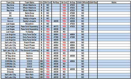
Hello. I created a filter that has 2 conditions. 1. If the Ref Cert or the SK Cert is YES, bit should appear. The problem is that if the columns with Ref Exp or SK Exp is blank, then it gives me a 0 or if it does have a date, then it gives me the number equivalent. The original table, it does have dates. I tried to format the columns so it would give me an actual date, but it doesn't work. It only works for the blank cells. This is the actual formula. =FILTER(C3:N500,((H3:H500)="YES")+((J3:J500)="YES"))&IF(ISBLANK(I3),"",I3) Array is C3 : N500 (This is the table where is information is coming from) Ref Cert is H3 : H500 SK Cert is J3 : J500 This is what the finish product looks like.427Views0likes5Comments
When #VALUE! isn’t an error: The hidden reference behavior of Excel’s dynamic arrays
1. Mechanism Overview Functions such as TAKE, DROP, OFFSET, and INDIRECT normally produce a range when supplied with scalar parameters. When instead a 1-D or 2-D numeric array is passed to one of these parameters, Excel attempts to generate multiple range outputs (one per array element). Since Excel’s grid architecture does not allow a single function call to return multiple ranges in parallel, the function fails. The visible result is an array filled with #VALUE!. Example patterns: =TAKE(range, {1;2;3;4}) =DROP(range, {1;2;3;4}) =OFFSET(range, {1;2;3;4}, {1,2,3}) =INDIRECT("A1:B"&{1;2;3;4}) Excel returns: { #VALUE!; #VALUE!; #VALUE!; #VALUE! } Although the values appear identical, each #VALUE! is associated with a distinct internal range reference corresponding to the attempted slice, offset or address. This is a side effect of Excel’s reference-binding layer, which attaches metadata to #VALUE! propagation structures when a reference-producing function fails after partially resolving its operands. 2. Behavior Characterization 2.1 Reference Retention Each #VALUE! error produced by the above functions contains a deferred reference representing the range the function attempted to construct. The reference is not materialized because: a multi-range return is not allowed, and the evaluation is aborted at the final conversion stage. However, the binding phase (operand resolution) has already created a reference object. This object is preserved internally and passed forward along the calculation chain. 2.2 Deferred Evaluation Functions that inspect operand values (e.g., SUM, MIN, COUNT) cannot extract data from these encapsulated #VALUE! tokens and will propagate the error. Functions that inspect operand references — such as MAP, SCAN, REDUCE, MAKEARRAY, and aggregation functions that re-evaluate their inputs individually — trigger evaluation at the point of consumption. Example: =MAP( TAKE(range, {1;2;3;4}), SUM ) In each MAP iteration: ref is a #VALUE! carrying an unresolved range reference. SUM(ref) requests value-level evaluation of that range. The reference is resolved at that moment only. The resulting scalar is passed downstream. Thus, the #VALUE! error acts as a strict thunk. 3. Functional Implications for Formula Construction 3.1 Range-Object Semantics The technique enables modeling of ranges as first-class reference structures, not arrays of extracted values. This allows: passing range slices through pipelines keeping intermediate objects lightweight avoiding large intermediate spillage reducing recalculation costs for multi-slice operations 3.2 Lazy Slice Evaluation Using {n1; n2; …} arrays in index parameters creates a vector of deferred slices. Functions downstream resolve these slices on demand and only for the specific iteration that needs them. This is especially useful for: sliding-window logic multi-pass transformations tree/graph-like iterative algorithms in Excel dynamic partitioning of ranges recursive constructions implemented with SCAN/REDUCE501Views2likes6Comments
GLSU Excel add-in fails to load after Office update from Version 2607 to 2608
Our Excel add-in, Process Runner GLSU , fails to load after Microsoft Office updates from Version 2607 to Version 2608. This started August 17, 2026 and is actively growing in scope. Error messages: Excel: Cannot run the macro 'onLoad' VBA: System Error &H80004005 (-2147467259). Unspecified error VBA: Compile error in hidden module: ThisWorkbook Has anyone encountered similar issue with their own custom add-on. If yes, any pointers to fix it. We are seeking help on priority. Thanks, Vrushali Pawale, Sr. Manager, Insightsoftware.551Views0likes1CommentDoes a LET variable get computed even if it's only referenced inside IFNA's fallback argument?
In the formula below, expensiveMatch is defined in LET but only referenced as IFNA's fallback argument: =LET( matchRow, XMATCH(1, (A1=Sheet2!$A$1:$A$1000)*(B1=Sheet2!$B$1:$B$1000)), x, INDEX(Sheet2!$C$1:$C$1000, matchRow), expensiveMatch, INDEX(Sheet3!$C$1:$C$500, XMATCH(A1&B1, Sheet3!$A$1:$A$500&Sheet3!$B$1:$B$500)), IFNA(x, expensiveMatch) ) Question: When x resolves successfully (no #N/A), does expensiveMatch still get computed because it's a top-level LET variable - or does Excel skip it since IFNA's fallback argument is never reached? I know IFNA short-circuits its fallback argument, and LET avoids recomputing a variable if referenced multiple times - but I haven't found much documentation on the behavior of Let. Is the below a more efficient way to write the formula? =LET( matchRow, XMATCH(1, (A1=Sheet2!$A$1:$A$1000)*(B1=Sheet2!$B$1:$B$1000)), x, INDEX(Sheet2!$C$1:$C$1000, matchRow), IF(ISNA(x), INDEX(Sheet3!$C$1:$C$500, XMATCH(A1&B1, Sheet3!$A$1:$A$500&Sheet3!$B$1:$B$500)), x ) ) Is this restructuring necessary, or does the first version already skip the unused computation? Basically I'm wondering if Let computes lazily/defers calculation in the way SQL's optimizer works. Input from anyone with insight or knowledge into the calc engine would be greatly appreciated. Thanks (Currently on Microsoft Excel for Microsoft 365 MSO (Version 2607 Build 16.0.20228.20190) 64-bit)591Views0likes10Comments