Forum Discussion
VBA Code to Automatically Copy and Paste a Range of Data if the Criteria is Met

 Mar 06, 2023
=IFERROR(INDEX(Sheet2!D$81:D$86,SMALL(IF(Sheet2!$F$81:$F$86>Sheet2!$G$81:$G$86,ROW(Sheet2!$A$81:$A$86)-80),ROW($A1))),"")Without VBA you can try this formula. The formula has to be entered as an arrayformula with ctrl+shift+enter if one doesn't work with Office 365 or Excel 2021. In the example the formula is in cell H2 of sheet8 and filled across range H2:K8.
Sheet2:
Sheet8:
One column contains a list and in another column is a SUMIF function that corresponds to the list column. I’m trying to use the function to only copy the values in that range where the SUMIF column has values “>0” and paste them on another sheet.
I’ve tried looking to see if other people have posted a similar question and gotten an answer but haven’t found anything replicable.
Again, I am open to a code that could automatically run as new data is added.
- OliverScheurichMar 12, 2023Gold Contributor
Could you attach a screenshot of your data (without sensitive information) and of the expected result?
 ABro_1111Mar 12, 2023Copper Contributor
Sure! So I've designed a simplified mockup and attached it for you. Hope it makes sense. But I'll explain it a bit more below.
On one sheet (named"Sidework") I have tons of data which is where my drop-down lists are derived from.
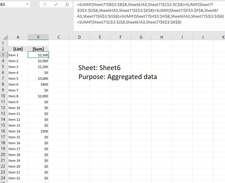
I then used another sheet named "Sheet6" to house data. The first column is a direct reference to the list from the "Sidework" sheet so that they are updated simultaneously. The second column contains the SUMIF formula
My summary sheet, "Sheet7" is where the values and data are updated. So for each person, I can select the item from the drop-drown list created, and insert how much they've earned from it. (This is what my SUMIF function is referencing.)
This is where I need help:
At another location on the same sheet, I want to display the data in another way. Showing the total earned per item rather than per person. But, I want excel to filter the data from Sheet6 and just copy and paste the range of data (just values and format) where the values in column B are greater than 0.So I tried to modify the function you gave me, by applying it to the data on Sheet6. But, I haven't had success (I think it's because the entire data set is technically a function.) Similar to the first example, my data is dynamic, so I need something that works with changing data.
*Note: I'm open to all suggestions as well. Thank you
- OliverScheurichMar 12, 2023Gold Contributor
Thank you for the detailed explanation. You can try this formula which must be entered as an arrayformula with ctrl+shift+enter if one doesn't work with Office 365 or Excel 2021.
=IFERROR(INDEX(Sheet6!A$3:A$1000,SMALL(IF(Sheet6!$B$3:$B$1000>0,ROW(Sheet6!$A$3:$A$1000)-2),ROW(Sheet6!$A1))),"")The formula is in cell E42 of Sheet7 and filled across range E42:F51. The formula can be filled down and the ranges in the formula can be adapted from e.g. Sheet6!A$3:A$1000 to Sheet6!A$3:A$20000.
An alternative could be these lines of code. In the attached file you can click the button in cell H38 of Sheet7 to run the macro.
Sub summary()

Dim i, j, k As Integer

Sheets("Sheet7").Range("H42:I1048576").Clear
j = Sheets("Sheet6").Range("A" & Rows.Count).End(xlUp).Row
k = 42
For i = 3 To j
If Sheets("Sheet6").Cells(i, 2).Value > 0 Then
Sheets("Sheet7").Cells(k, 8).Value = Sheets("Sheet6").Cells(i, 1).Value
Sheets("Sheet7").Cells(k, 9).Value = Sheets("Sheet6").Cells(i, 2).Value
k = k + 1
Else
End If

Next i

End Sub
In cell B3 of Sheet6 i've entered a shorter formula which must be entered as an arrayformula with ctrl+shift+enter if one doesn't work with Office 365 or Excel 2021. The ranges of the formula can be adapted as required.
=SUM(IF(Sheet7!$B$3:$J$8=Sheet6!A3,Sheet7!$C$3:$K$8))