Forum Discussion
Excel Formula
Hi,
i want to list the 5 most frequented numbers in a column of my excel sheet top down. could anyone give me an idea about the right formula?
Let's say the numbers are in A2:A101.
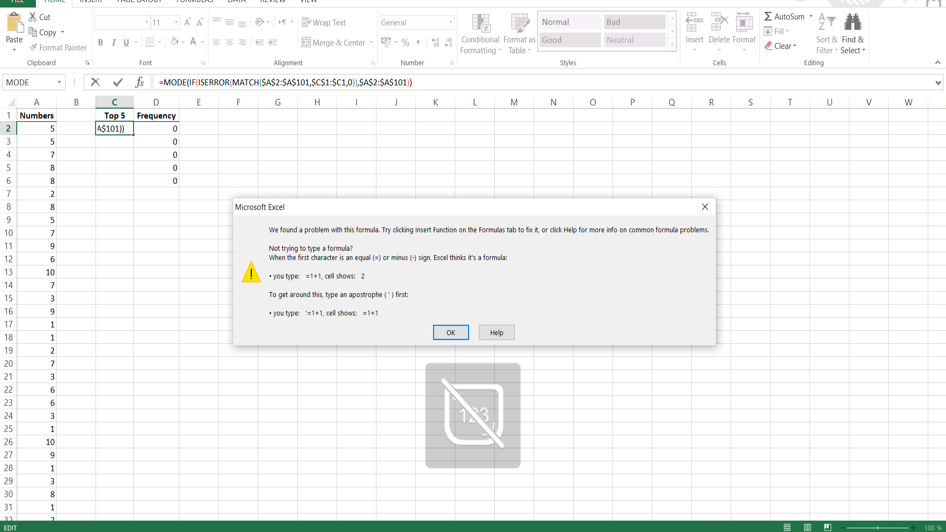
In C2, enter the formula
=MODE(IF(ISERROR(MATCH($A$2:$A$101,$C$1:$C1,0)),$A$2:$A$101))
and confirm it with Ctrl+Shift+Enter to turn it into an array formula (this is essential!)
Fill down to C6.
See the attached sample workbook.
18 Replies
- SergeiBaklanDiamond Contributor
And on 365
=LET( freq, FREQUENCY(numbers,numbers), skipLast, INDEX(freq, SEQUENCE(ROWS(freq)-1)), topN, SEQUENCE(5), topNumbers, INDEX(SORTBY(numbers,skipLast,-1),topN), topFreq, LARGE(SORT(skipLast,,-1),topN), IF({1,0}, topNumbers, topFreq) ) BabakGhadiriCopper ContributorHi Sergei !
you sent me already a formula about the 5 Top most repeated numbers in a column in excel. This was very useful for me. Just another question. when i fill down the column C , it shows till Row 11 and afterwards shows #N/A . how can i make it show the rest numbers down without limit ? or may be you send me a new formula without this limit?
Thanks already- SergeiBaklanDiamond Contributor
- BabakGhadiriCopper ContributorThank you a lot, this was useful.
- Detlef_LewinSilver Contributor
With ties:
=LET( unique, UNIQUE(numbers), count, COUNTIFS(numbers,unique), sort, SORTBY(IF({1.0},unique,count),count,-1), sorted_count, INDEX(sort,0,2), include, sorted_count>=LARGE(sorted_count;5), FILTER(sort,include) )- SergeiBaklanDiamond Contributor
Exactly, if only correct misprints for English version
=LET(
  unique, UNIQUE(numbers),
  count, COUNTIFS(numbers,uniq),
  sort, SORTBY(IF({1},unique,count),count,-1),
  sorted_count, INDEX(sort,0,1),
  include, sorted_count>=LARGE(sorted_count,5),
  FILTER(sort,include)
)
and add frequency to the result
- Detlef_LewinSilver Contributor
With a pivot table:
Numbers column in rows area and in values area. Change from Sum to Count.
Sort values column in descending order.
Set a Top10 filter for the Numbers column.
Let's say the numbers are in A2:A101.
In C2, enter the formula
=MODE(IF(ISERROR(MATCH($A$2:$A$101,$C$1:$C1,0)),$A$2:$A$101))
and confirm it with Ctrl+Shift+Enter to turn it into an array formula (this is essential!)
Fill down to C6.
See the attached sample workbook.
- BabakGhadiriCopper ContributorHi Hans !
you sent me already a formula about the 5 Top most repeated numbers in a column in excel. This was very useful for me. Just another question. when i fill down the column C , it shows till Row 11 and afterwards shows #N/A . how can i make it show the rest numbers down without limit ? or may be you send me a new formula without this limit?
Thanks alreadyChange the formula to
=IFERROR(MODE(IF(ISERROR(MATCH($A$2:$A$101,$C$1:$C1,0)),$A$2:$A$101)),"")
- BabakGhadiriCopper ContributorThanks a lot, it was useful.
- BabakGhadiriCopper Contributor
Column D simply uses COUNTIF to return the frequency of the number in column C.
The formula in C2 calculates the most frequently occurring number, that in C3 the second most frequently occurring number etc. These formulas only refer to column A, not to column D.