Forum Discussion
Excel Formula
- May 21, 2021
Let's say the numbers are in A2:A101.
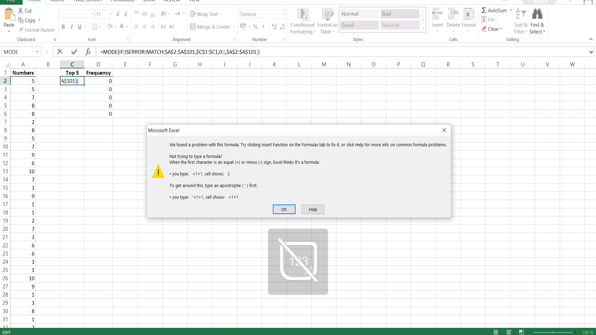
In C2, enter the formula
=MODE(IF(ISERROR(MATCH($A$2:$A$101,$C$1:$C1,0)),$A$2:$A$101))
and confirm it with Ctrl+Shift+Enter to turn it into an array formula (this is essential!)
Fill down to C6.
See the attached sample workbook.
Let's say the numbers are in A2:A101.
In C2, enter the formula
=MODE(IF(ISERROR(MATCH($A$2:$A$101,$C$1:$C1,0)),$A$2:$A$101))
and confirm it with Ctrl+Shift+Enter to turn it into an array formula (this is essential!)
Fill down to C6.
See the attached sample workbook.
Thanks,
but i do not know what is wrong with my sheet, it does not work on my sheet, instead it pops up an error. i sent the screen shot to you, could you please check it.
- HansVogelaarMay 21, 2021MVP
Column D simply uses COUNTIF to return the frequency of the number in column C.
The formula in C2 calculates the most frequently occurring number, that in C3 the second most frequently occurring number etc. These formulas only refer to column A, not to column D.