Forum Discussion
Some help with conditional formatting
Hey folks. Here's the scenario I have. I have two sheets open; in sheet2 I would like cell A1 to change colour if any cell in a range in sheet1 contains a certain value, eg. cat. I had done this in Google Sheets using the following formula: =not(iserror(vlookup("cat",indirect("sheet2!A1:A20"),1,false))) But it doesn't seem to work in Excel and I can't quite figure out why this formula results in a false output. I have verified that the range does contain the value it's looking for. Any suggestions are appreciated.
4 Replies
- Juliano-PetrukioBronze Contributor
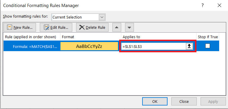
If the value you are looking for is on A1 youc an use this formula on conditional formatting
=MATCH(A1,sheet2!A1:A20,0) MrVmathsCopper Contributor
Juliano-Petrukio Thanks for your response. Unfortunately, the cell I want to be formatted doesn't contain the same thing that I want it to search for.
- Juliano-PetrukioBronze Contributor
It doesn't matter.
You just need to update the range or cell where you want the formatting to be applied.