Return the Cell(s) with the Highest SUM() between groups of Cells

I think you're on the right track with SUMIF and MAX. You just need to incorporate UNIQUE and FILTER to return the item(s) with the maximum total. In the event of ties, you may also want to consider using SORT and ARRAYTOTEXT to consolidate the list of items.

The following is just one example of a possible solution using a custom LAMBDA function:

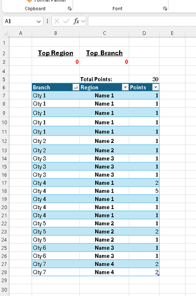
= TopInλ(Table25[[#All],[Region]], Table25[[#All],[Points]])

Where TopInλ is defined in Name Manager as:

= LAMBDA(field,values,[_0123],
    LET(
        k, UNIQUE(SORT(DROP(field,1))),
        i, SUMIF(field,k,values),
        j, MAX(i),
        x, CHOOSE(1+_0123,{1;3;4},{1,3,4},{1,3;2,4},{1,2;3,4}),
        CHOOSE(x,"Top "&TAKE(field,1),"Total",ARRAYTOTEXT(FILTER(k,i=j)),j)
    )
)

The optional [_0123] argument can be set to 1, 2 or 3 (default is 0 if omitted) to change the orientation of the final output. For example:

= TopInλ(Table25[[#All],[Region]], Table25[[#All],[Points]], 1)

The same formula can also be applied to the Branch field (or any other applicable field):

= TopInλ(Table25[[#All],[Branch]], Table25[[#All],[Points]], 1)

Please note, the function has been written to read the column header/label from the field reference, so you must include the header row when selecting the table column.

If you don't like any of the output options demonstrated here, or would prefer not to use a function defined in Name Manager, you could also just write the entire thing with your desired output using a single LET statement. For example:

= LET(
    TopIn, LAMBDA(field, LET(
        k, UNIQUE(SORT(DROP(field,1))),
        i, SUMIF(field,k,Table25[[#All],[Points]]),
        j, MAX(i),
        HSTACK("Top "&TAKE(field,1)&{":";" Total:"}, VSTACK(ARRAYTOTEXT(FILTER(k,i=j)),j))
    )),
    VSTACK(TopIn(Table25[[#All],[Region]]), TopIn(Table25[[#All],[Branch]]))
)

The same idea could also be achieved using GROUPBY instead of SUMIF:

= LET(
    TopIn, LAMBDA(field, LET(
        k, GROUPBY(field,Table25[[#All],[Points]],SUM,1,0),
        i, DROP(k,,1),
        j, MAX(i),
        HSTACK("Top "&TAKE(field,1)&{":";" Total:"}, VSTACK(ARRAYTOTEXT(FILTER(TAKE(k,,1),i=j)),j))
    )),
    VSTACK(TopIn(Table25[[#All],[Region]]), TopIn(Table25[[#All],[Branch]]))
)

Please follow-up with additionl questions, if needed. Cheers!