#ref error using If and Vlookup

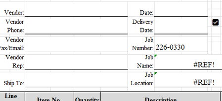
SEWRUN wrote:

=IF(H13>=@'[Job Status.xlsx]Sheet1'!$A$2:$A$1048576, VLOOKUP(H13,'[Job Status.xlsx]Sheet1'!$A$2:$A$1048576,2,),"")

I think that the formula is incorrect for two reasons:
. as OliverScheurich​ wrote, you don't have the 2nd column to retrieve data and is better to set FALSE or 0 as last parameter;
. the criteria H13>=@'[Job Status.xlsx]Sheet1'!$A$2:$A$1048576 return only H13>='[Job Status.xlsx]Sheet1'!$A$2, because the implicit intersection

@

grab the first value in range A2:A1048576 (that could be written as A:A at this point) and this is the reason, if not present, of #spill error and which means you are using a version higher than 2019 ;

Unfortunately, the sheet references are not visible in the image, but your request:

SEWRUN wrote:

if I put in the job number in H13 and it looks up the job in the other sheet that has all the jobs listed, it will return the name of the job and the location of the job

can be solved with:

=IFERROR(VLOOKUP(H13,'[Job Status.xlsx]Sheet1'!$A:$B,2,0);"Job not found")

or

=XLOOKUP(H13,'[Job Status.xlsx]Sheet1'!A:A,'[Job Status.xlsx]Sheet1'!B:B,2,0);"Job not found")

if you are using 365, use the trimrange notation:

=XLOOKUP(H13,'[Job Status.xlsx]Sheet1'!A:.A,'[Job Status.xlsx]Sheet1'!B:.B,2,0);"Job not found")

using dot after colon to stop range at last valued cell, in both cases, XLOOKUP manage the error with 4th parameter.
Change the references in formula to retrieve other column values.

Bye.