Forum Discussion
Highlighting alternate rows using conditional formatting
Hi all,
I am constructing a simple personal budget (Income, expense) excel sheet, and listing my expenses on a daily basis. I am hoping to highlight the rows based on alternate days for easy reference, for e.g. expenses on Aug 10 will be highlighted, and Aug 11 will not be and as follows....
<Rough idea of
Column B - Day (For e.g. Aug 10, Aug 11, as follows)
Column C - Activity (Lunch, etc)
Column D - Amount
Can anyone help with the formulas for conditional formatting or any alternative way to achieve it? It would be great if you would also give an explanation for it, thank you!!!
10 Replies
 Walter_PekCopper Contributor
The formulas provided is applicable if each days has 1 row, what if i have multiple rows for specific days. For e.g. Aug 9: 2 rows, Aug 10, 5 rows, etc..
 KodipadyIron Contributor
=ISODD() or ISEVEN() on date field will work. it will show all rows in same color for specific date.
have you checked this yet ?
- Walter_PekCopper Contributor
- PeterBartholomew1Silver Contributor
If your dates are proper date values rather than text strings, then 'weekend?' defined as
= WEEKDAY(thisDate,2)>5
could be used to conditionally format the weekends which could be more informative than an alternating pattern.
By the way, I agree with the earlier post that recommends the use of a table. Besides the normal alternating stripes it is possible to set that up with a 5rows/2rows repeat pattern.
- SergeiBaklanDiamond Contributor
By the way, it depends on how you'd like to design the table. Sometimes even with tables it is used CF with =MOD(ROW(),2)=0 or like, especially if to give different accents on different columns.
- PeterBartholomew1Silver Contributor
Can you think of anything else that might go in here ! 🙂
Mind you, I wish conditional formatting worked properly with Named Ranges and Arrays. You apply the format to a range by name and CF kindly replaced it with the usual direct reference junk (that description is only my opinion). What is true is that editing the sheet then scrambles the CF range. Again, if you have an array formula that you wish to use to format the output range, CF only recognises the lead element.
p.s. Just checked, CF seems to work better with Tables.
Hi
To apply banded rows conditional formatting:
- Select the range to format
- Home Tab >> Conditional Formatting >> New Rule
- Use Formula
- The formula I used is : =MOD(ROW(),2)=1
since the ROW function returns an incremental number >> I divide it by 2 (the divisor) and the MOD returns the REMAINDER 1,0,1,0,1,0... so the formatting will pop up if it is =1
This function works in list or tables.
It works also for Banded columns but replace ROW() by Column()
Hope that Helps
Nabil Mourad
- KodipadyIron Contributor
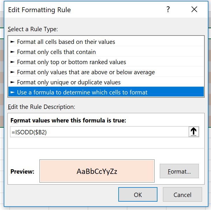
You can use formula
=ISODD($B2)
This will be true or false for alternating days. you can also use ISEVEN() function.
Please look at the pictures attached for details.
- Subodh_Tiwari_sktneerSilver Contributor
Why not convert the data into an Excel Table and you will have the desired layout without any conditional formatting?
Select one cell in your data and press Ctrl+T and in the new popped up Create Table confirmation window, check the CheckBox next to "My table has headers" and click OK to finish.
Once your data is converted into an Excel Table and any cell is still selected in the Table, you will find a new tab called "Table Design" and there you can change the different Table Style if you don't like the default style.
Table Design Tab will only appear on the Ribbon if you select any cell in the table.