Forum Discussion

Dynamic table

=LET(_pulled,IFNA(REDUCE({"Profile"."Number"."Step"."Torque"."Position"},VSTACK(Mastersheet!B2:.B10),
LAMBDA(u,v,VSTACK(u,HSTACK(v,XLOOKUP(v,Mastersheet!B2:.B100,Mastersheet!C2:.C100,""),
FILTER(INDIRECT("'"&v&"'!A2:C100"),INDIRECT("'"&v&"'!A2:A100")<>""))))),""),
HSTACK(_pulled,VSTACK("Sequence",SEQUENCE(ROWS(_pulled)-1))))
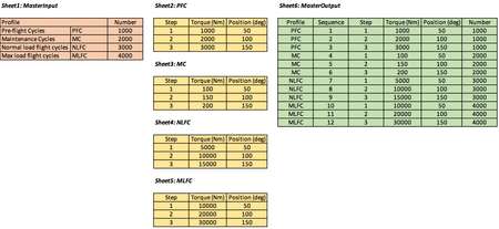
It's perhaps impossible with 'just normal' Excel functions. But with Microsoft 365 we can built something dynamic that pulls the results if all tables are in range A1:C100 in their sheets. The headers are always in range A1:C1 in my example.
- m_tarlerOct 08, 2026Silver Contributor
I would recommend you convert all of those input table to be tables and name them according to their profile name so you can directly pull the data (using indirect) using the profile name. Here is the same output from OliverScheurich but using table names (I also defined MIP and MINu for the MasterInput Profile column and the MasterInput Number column so the REDUCE loop didn't have to query them each time:
=LET(MIP,MasterInput[Init],MINu,MasterInput[Number],
_pulled,IFNA(REDUCE({"Profile","Number","Step","Torque (Nm)","Position (deg)"},MIP,LAMBDA(p,q,
                 VSTACK(p,HSTACK(q,XLOOKUP(q,MIP,MINu),INDIRECT(q))))),""),
HSTACK(_pulled,VSTACK("Sequence",SEQUENCE(ROWS(_pulled)-1))))
so what is the big change? basically in the original formula was
FILTER(INDIRECT("'"&v&"'!A2:C100"),INDIRECT("'"&v&"'!A2:A100")<>"")
and now by using tables it is
INDIRECT(q)
note that q is the same as v in the original formula.
So how does that work? If you highlight the table or even just click in the table area and then go to HOME->Format as Table and then select any color scheme you want. In the pop-up you should see the table range highlighted and the second row asks about a name, change that to the profile name. Make sure 'has headers' is checked. then say ok. That will then create a NAME for that table range and that range will expand and contract as you add or delete from the table. In the new formula you can see I defined the table on the MasterInput sheet the same was and can reference the individual columns of that table using for example MasterInput[Init] because I named the column with the profile initials as Init.
on another note,
I also modified it a bit to repeat the profile initials and the Numbers and be in the requested column order:
=LET(MIP,MasterInput[Init],MINu,MasterInput[Number],
 REDUCE({"Profile "," Sequence "," Step "," Torque (Nm) "," Position (deg) "," Number"},MIP,LAMBDA(p,q,
   LET(t,INDIRECT(q),b,EXPAND("",ROWS(t),,""),
       VSTACK(p,HSTACK(q&b,SEQUENCE(ROWS(t),,N(INDEX(TAKE(p,-1),1,2))+1),t,XLOOKUP(q,MIP,MINu)&b)))))
)
And I will try to attach my sample sheet for you and if others want to put in their options. Both of the above formulas are shown on the MasterOutput sheet
