excel
45098 Topics
#ref error using If and Vlookup
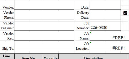
I'm trying to use this formula with the IF and Vlookup =IF(H13>=@'[Job Status.xlsx]Sheet1'!$A$2:$A$1048576, VLOOKUP(H13,'[Job Status.xlsx]Sheet1'!$A$2:$A$1048576,2,),"") The idea is, if I put in the job number in H13 and it looks up the job in the other sheet that has all the jobs listed, it will return the name of the job and the location of the job. I've used this formula to connect other sheets to this 'job status' workbook and it works fine. I don't understand why it is not working here. If I remove the @ symbol from the beginning of the formula, it makes it a #spill! error. In my other workbooks where this formula works, I didn't have to put the @ sign in. Thank You.61Views0likes2Comments
Excel Nested Arrays: Find the Nesting Depth of Uniform and Ragged Arrays ARRDEPTH() & ISRAGGED()
Hey everyone! I’ve been diving deep into Excel’s new nested arrays features lately, and I absolutely love the flexibility they bring to data structuring. However, managing them can get a bit tricky, so I figured I’d build some specialized tools to handle them seamlessly. Public Interfaces & Arguments =ISRAGGED(array) Argument Description Default Behavior array Target nested structure to validate. Required =ARRDEPTH(array, [is_ragged]) Argument Description Default Behavior array Target nested structure to measure. Required [is_ragged] TRUE: Scans all branches for the deepest path. FALSE: Speed test on the first path only. FALSE (Omitted) TL;DR (What makes it tick): Function Name Type What It Does ARRDEPTH Public UI Returns nesting depth. Supports deep checking or fast linear testing. ISRAGGED Public UI Structural validator. Returns TRUE if array branches have uneven nesting. ANALYZE_NESTING Hidden Core Engine Multi-process recursive parser that tracks tree structure geometries. LINEARDEPTH Hidden Utility High-speed depth checker that evaluates the first element path exclusively. You can get both functions from my GitHub Gist: https://gist.github.com/Medohh2120/9cdf939036942c9672c57ccd6de696d3104Views0likes4CommentsExcel pivot chart's secondary axis disappears after parameter in chart is filtered at slicer
Hi, A pivot chart on Sales (primary y axis) and Rate (secondary y axis) is plotted against time (X axis). Area parameter is part of the underlying dataset, but not plotted in same chart. When Area or Rate is filtered at respective slicer, the secondary y axis disappears i.e. pivot chart resets to having only primary y axis How may I keep the secondary y axis after filtering? Thank you.1.1KViews0likes6Comments
Excel can still use legacy “Move and Size with Cells” checkboxes — but can no longer create them
Excel Can Still Use “Move and Size with Cells” Form Checkboxes — But It Can No Longer Create Them A reproducible Excel compatibility regression hiding inside legacy Form Controls For years, I have used Excel workbooks containing hundreds of Form Control checkboxes attached to product rows. These checkboxes behaved exactly as you would expect: - change the row height, and the checkbox stays inside that row; - filter the worksheet, and the checkbox disappears together with its product; - remove the filter, and the checkbox returns to the correct row; - no overlapping controls; - no “click one checkbox, activate another” behaviour. Recently, while rebuilding one of these workbooks in Excel 2024 LTSC, I discovered something very strange. The old checkboxes still work perfectly. But if I delete one and recreate it — even using the same VBA code that originally created the controls — Excel creates a different kind of placement behaviour. After a full day of controlled testing, XML inspection and A/B workbook comparison, the problem became clear: Excel can still read, display, save and execute legacy Form Control checkboxes using true “Move and size with cells” behaviour — but current Excel cannot recreate that same state for a newly created Form Control checkbox through the normal UI or VBA object model. That is not just inconvenient. For existing business workbooks, it is a serious backward-compatibility problem. The simple VBA code that used to work The original controls were created with ordinary Excel VBA: Set myCBX = wks.CheckBoxes.Add( _ Top:=cell.Top, _ Left:=cell.Left, _ Width:=cell.Width, _ Height:=cell.Height) Nothing exotic. No custom event engine. No ActiveX. No external add-in. Just a standard Excel Form Control checkbox positioned exactly over a cell. The workbook contains roughly 1,000 of these controls. The old ones still behave correctly today. The problem starts only after deleting them and creating new ones. What changes? In the Excel UI, the difference is immediately visible. For an original legacy checkbox: Format Control → Properties shows: Move and size with cells The option is selected, although it is greyed out. For a newly created checkbox in current Excel: Move but don’t size with cells is selected instead. That already suggests something changed internally. But the real evidence is inside the .xlsm package. The OOXML tells the story I created two controlled test workbooks: Workbook A Original legacy Form Control checkboxes that behave correctly. Workbook B The same workbook, but the checkboxes were deleted and recreated in current Excel using the original VBA logic. The internal OOXML differs. The working legacy controls contain placement information equivalent to: moveWithCells="1" sizeWithCells="1" and use genuine two-cell anchoring. The newly generated controls are instead stored using one-cell-style placement semantics, including: <xdr:twoCellAnchor editAs="oneCell"> The important part is not merely the XML syntax. The resulting behaviour is observably different. With the legacy control, both ends of the object are anchored to the worksheet grid. With the newly created control, Excel effectively preserves the control size while cells move underneath it. That distinction becomes disastrous when rows are resized, hidden or filtered. Why filtering exposes the problem Imagine a checkbox sitting on row 50. With the legacy behaviour: Checkbox ↔ Row 50 boundaries When row 50 changes size, the checkbox changes with it. If row 50 is filtered out, the control disappears with the row. When the row becomes visible again, the control is still exactly where it belongs. With the newly generated control, its dimensions are not tied to both cell boundaries in the same way. After repeated resizing and filtering, controls can begin to overlap. That leads to one of the worst possible spreadsheet UI failures: You click the checkbox you can see, but another checkbox receives the click. For a workbook containing hundreds or thousands of rows, this makes the controls unreliable. “Just use .Placement = xlMoveAndSize” That was the obvious first solution. Excel VBA defines: xlMoveAndSize as the placement mode where an object moves and resizes with cells. So I tested: myCBX.Placement = xlMoveAndSize and: myCBX.Placement = 1 I also tested placement through the corresponding Shape: ws.Shapes(myCBX.Name).Placement = xlMoveAndSize And through a ShapeRange. And through DrawingObjects. And even the commonly suggested workaround: Group controls → set Group.Placement = xlMoveAndSize → Ungroup None of these recreated the original internal state in Excel 2024 LTSC. The workbook continued to serialize the new controls differently. This matches long-standing Microsoft guidance that Form Control checkboxes do not normally support “Move and size with cells” as an editable option, while ActiveX checkboxes do. And yet — this is the important part — existing legacy Form Control checkboxes in real workbooks can still possess and use that state. The most revealing experiment I then modified the OOXML manually. I took the newly generated workbook and patched the checkbox placement metadata to match the working legacy controls: moveWithCells="1" sizeWithCells="1" with proper two-cell anchoring and without the one-cell override. Then I reopened the workbook in Excel 2024 LTSC. And it worked. Immediately. No custom VBA reposition engine. No ActiveX. No workaround running continuously. The same Excel installation that would not create this state through VBA had absolutely no problem: - reading it, - displaying it, - saving it, - resizing the controls with rows, - and filtering them correctly. That is the key finding. The Excel rendering and file engines still fully understand this checkbox state. The missing part is the supported creation path. So is this an unsupported feature or a compatibility regression? Microsoft has historically documented Form Control checkboxes as not supporting “Move and size with cells” in the normal UI. That makes the situation unusual. The issue is not simply: “Excel removed a documented checkbox feature.” The stronger and more accurate statement is: Excel supports a legacy Form Control state in existing workbooks, continues to execute it correctly, but no longer provides an ordinary supported mechanism to reproduce that same state for a replacement control. For users maintaining long-lived Excel systems, the difference is academic. If an old control is accidentally deleted, replacing it with an apparently identical Form Control changes the behaviour of the workbook. That is a backward-compatibility problem. Why not switch to ActiveX? ActiveX checkboxes support richer placement behaviour. But that creates another problem. Microsoft now disables ActiveX controls by default in Microsoft 365 and Office 2024 for security reasons. When ActiveX is disabled, users cannot create new ActiveX objects or interact with existing ones. So the official alternatives are hardly attractive: Legacy Form Controls Lightweight and reliable — but cannot reproduce this legacy placement state normally. ActiveX Supports more control behaviour — but is now a legacy security-sensitive technology disabled by default in current Office. New in-cell checkboxes Architecturally much better — because the checkbox is part of the cell and represents TRUE/FALSE. But Microsoft’s own documentation currently lists the feature for: - Excel for Microsoft 365 - Excel for Microsoft 365 for Mac not Excel 2024 LTSC. That leaves perpetual Office users in an uncomfortable middle ground. This is where the product story becomes difficult to defend I am not claiming that Microsoft intentionally removed this behaviour in order to sell subscriptions. There is no evidence for that claim. But the resulting user experience is still hard to justify: 1. Excel can execute the legacy checkbox behaviour. 2. Excel can preserve it. 3. Excel can save it. 4. Excel accepts a manually patched workbook containing it. 5. Excel’s current object model does not provide a reliable way to recreate it. 6. The modern replacement — native in-cell checkboxes — is documented for Microsoft 365 rather than Excel 2024 LTSC. 7. The other legacy alternative, ActiveX, is now disabled by default for security reasons. For users maintaining mature Excel applications, this is a poor migration path. Why this matters beyond checkboxes This is not really a story about one checkbox property. It is about the contract users expect from long-lived productivity software. Excel workbooks are often not disposable documents. They can be: - product-management systems, - pricing tools, - engineering calculators, - operational forms, - purchasing systems, - inventory tools, - reporting applications, - or business processes maintained for ten or twenty years. When Excel continues to support the execution of an old document feature but silently prevents users from recreating an equivalent object, maintaining those systems becomes unnecessarily difficult. Backward compatibility should mean more than: “The file still opens.” It should also mean: “A user can maintain the workbook without reverse-engineering its OOXML package.” What Microsoft could do There are several reasonable fixes. Option 1 — Restore proper placement support Allow: CheckBox.Placement = xlMoveAndSize to generate the same placement state that Excel already understands for legacy controls. Option 2 — Expose the existing capability If the engine already supports it, expose “Move and size with cells” again for Form Control checkboxes. Option 3 — Provide a migration path Make the new in-cell checkbox functionality available to perpetual Excel releases as well, or provide an official conversion tool from legacy Form Controls to cell checkboxes. Option 4 — At minimum, document the limitation If this legacy state is intentionally read-only for compatibility, document it clearly. Currently, a user can spend hours debugging VBA without realizing that two visually identical Form Control checkboxes can have fundamentally different internal placement semantics. A workaround exists — but users should not need it The workaround I eventually used was to modify the .xlsm OOXML package so that newly generated controls use the same anchor metadata as the working legacy controls. That solved the problem immediately. But manually patching Office XML should not be necessary to restore behaviour that Excel itself already supports. It is a useful proof of concept. It is not an acceptable product-level solution. The reproducible evidence I have retained minimal A/B test workbooks demonstrating the problem: OLD Original Form Control checkboxes with correct legacy placement. NEW The same workbook after deleting and recreating the controls. The differences can be reproduced and inspected directly in the workbook OOXML. I would be happy to provide the files to Microsoft Excel engineering. Final thought Excel’s reputation was built partly on extraordinary backward compatibility. That is why companies still trust .xls and .xlsx files created years — sometimes decades — ago. This case shows an uncomfortable edge of that compatibility: Excel remembers how to use an old feature, but appears to have forgotten how to create it. When the workaround is to unzip an .xlsm, manually alter OOXML placement records, rebuild the package and reopen it in Excel — and Excel then works perfectly — it is difficult to argue that the capability itself is gone. The engine still knows how. The user simply no longer has a supported button or VBA path to ask for it. Microsoft, please give that capability back — or provide a proper migration path. Sources Microsoft documentation for native cell-based checkboxes: https://support.microsoft.com/en-us/excel/using-check-boxes-in-excel Microsoft-hosted discussion on Form Control checkbox limitations: https://learn.microsoft.com/en-us/answers/questions/4813119/is-there-a-way-to-assign-a-checkbox-to-a-cell Microsoft documentation on ActiveX controls being disabled by default: https://support.microsoft.com/en-us/office/vba/activex-controls-are-disabled-by-default-in-microsoft-365-and-office-2024169Views0likes3CommentsPut multiple values in one cell with lists and arrays in Excel
Throughout Excel's 40-year history, you've only been able to put one value per cell. In this announcement, we're excited to share how that's changing with the release of lists, arrays in cells, and nested arrays, initially to Microsoft Excel for Windows and Mac Beta Channels. Many workbooks already try to pack multiple values into one cell. A project might list "Carlos, Henrietta, Jacob" as three owners, or a Forms survey might return "2:00 PM; 2:30 PM; 3:00 PM" as one response. With lists, you can keep those values in one cell, while also keeping them separate for filtering, calculation and more. Later in this post, we'll explore arrays in cells and nested arrays in more depth. NOTE: These are preview features. Their behavior may change before general release based on your feedback. We don't recommend using them in important workbooks until they're generally available. Lists Lists let you put multiple values into one cell. You can create a list by selecting Insert > List or pressing Ctrl+J, then typing or pasting items separated by commas or semicolons, depending on your regional settings. Selecting the icon in the cell shows the individual values. You can add, remove, or edit list items by double-clicking the cell or pressing F2, just like other values. With lists, you can filter by one or more individual items instead of whole text entries. Referencing a list returns all its values for calculations. For example, =B2 spills those values into separate cells. Arrays in cells Lists are useful on their own, but they're part of a much broader change to Excel. For the first time in Excel, arrays can exist natively in cells as values or as formula results. They can be any size or shape and can even contain other arrays. You can now keep the result of any spilling formula in a single cell by "wrapping" the formula body with braces { }. Since the introduction of dynamic arrays, array results have spilled across cells – for example ={1;2;3}. Wrapping the original array with braces creates a 1x1 array around it, so instead of spilling to multiple cells, the array stays in a single cell. Braces have long been used to describe arrays in Excel and this extends that behavior by allowing multiple layers of braces. This gives you more flexibility when building spreadsheets. Instead of leaving room for a formula to spill, you can keep the result in one cell. Arrays inside arrays, or nested arrays Arrays can now also "nest" inside other arrays. For example: ={{1,2,3};{4,5,6}} Previously, a formula that produced an array of arrays would return a truncated result or #CALC! error. Now, supported formulas return the complete nested result. In the example below, you can see how TEXTSPLIT behaves with and without nested arrays. Without nested arrays, Excel only returns the first item for each row. With nested arrays, the result spills, one array per row. The arrays in each row can then be used in further calculations. Four new functions: FLATTEN, HAS, HASANY, HASALL To help you work with arrays more easily, we've added four functions. FLATTEN(array, [pad_value], [levels]) simplifies nested arrays by removing one or more levels of nesting. Continuing from the prior example, FLATTEN lets you simplify the nested array output, spilling the individual results into the grid. We used an empty string ("") for pad_value so rows with fewer items show blanks in the remaining columns. Three HAS functions check whether values are in an array: HAS(array, value) returns TRUE if value appears anywhere in array, and FALSE otherwise. HASANY(array, values) returns TRUE if any of the values appear anywhere in array, and FALSE otherwise. HASALL(array, values) returns TRUE if all of the values appear anywhere in array, and FALSE otherwise. Do more with spreadsheets using arrays in cells and nested arrays Arrays in cells open up spreadsheet designs that weren't practical before. The run tracker below captures split times (how long it takes to run each kilometer) in a table with one run per row. The number of splits depends on the length of the run. Stats for each run are calculated right in the same table. For more examples, I recommend looking to your favorite Excel communities on LinkedIn, YouTube, Reddit, or elsewhere. Enabling nested array calculations in a workbook Compatibility Version 3 will be released alongside arrays in cells and is required for most calculations involving nested arrays. You can set Compatibility Version for each workbook in by selecting Formula > Calculation Options. See compatibility versions for more information. Some existing formulas return different results in Compatibility Version 3. If your workbook doesn't behave as expected, you can keep it set to Compatibility Version 1 or 2. Known limitations As this feature rolls out to Beta Channel, the following limitations apply: Conditional formatting doesn't inspect array contents unless you use a formula Data validation can't use a list or array as dropdown items Charts don't expand an array into data points PivotTables don't read array values as source data Power Query doesn't load or emit array-valued columns Find & Replace can't replace list/array items Availability These improvements are rolling out to Beta Channel users running: Windows: Version 2610 (Build 20520.20000) or later Mac: Version 16.114 (Build 26092111) or later Features covered on this blog roll out over time to enable us to monitor quality and performance, so some preview features may not be available to you right away. Also note that features may be paused, adjusted, or removed as part of that process. Feedback Click Help > Feedback in Excel to tell us what you think.37KViews14likes54CommentsExcel x64/VBE event entry loses execute permission in the default segment heap
Excel x64/VBE event entry loses execute permission in the default segment heap; reproduced after Office update Please route to the Office VBA runtime team and Windows heap team. We need a supported runtime fix or deployment workaround, not DEP/ASLR disablement or VBA page-permission patching. Environment: Windows 11 Pro 25H2 build 26200.9457; ntdll 10.0.26100.9278. Excel x64 16.0.20430.20140 updated through official Click-to-Run to 16.0.20430.20146. VBE7.DLL remains 7.1.11.58, unchanged SHA256; Microsoft signatures Valid. Retail Office 2021 + Project 2024. No heap override or disabled mitigations. A fresh native blank workbook (15 blank sheets, counters/empty document-method bodies) plus ordinary GetProcessHeap/HeapAlloc/HeapFree DATA allocations reproduces the same execute AV seen in our business workbook. No PMS business implementation, save/protection logic, project data, license logic, userform, custom executable buffers or permission-writing APIs are present in the minimal fixture. After the update, the SAME isolated repro ran with CDB attached. All generated VBE entries were initially executable. A paired entry/return of the SAME NtAllocateVirtualMemoryEx call recorded base 0x1b8ef147000, size 0x3c000, MEM_COMMIT, PAGE_READWRITE. The live VBE entry page 0x1b8ef166000 changed from protection 0x40 to 0x04. !heap -x confirmed the allocation was still LFH Allocated (requested 4144, block 4352), with entry bytes intact. A normal Worksheets.Add then delivered Workbook_NewSheet and faulted at 0x1b8ef166dc4: C0000005, Parameter[0]=8. Stack includes DispCallFuncAmd64, VBE7 EpiInvokeMethod and EVENT_SINK_Invoke. The permission-change stack is RtlAllocateHeap -> LFH subsegment reformat -> SegLfhVsCommit -> SegPageRangeCommit -> SegMgrCommit -> NtAllocateVirtualMemoryEx. An earlier minimal run and the original/freshly rebuilt business project also showed this mechanism. Rebuilding VBA compilation state did not remove it. Traditional-heap business/save smoke acceptance passed, but that is not a portable commercial fix. Limitations: the compact fixture has reproduced with CDB attached; two no-debugger minimal runs were negative. We do not claim universal impact or an already accepted Microsoft bug. Heap documentation warns against executable permission changes on heap allocations, so ownership of the VBE/heap interaction requires vendor assessment. Reviewed minimal workbooks/source and sanitized paired traces are available in a small technical package. No real project, license credentials, private keys, Microsoft DLLs or full dump will be uploaded. Please advise: (1) supported VBE allocation/protection behavior; (2) serviced runtime/Windows build fixing this precise mechanism; (3) supported administrator-deployable mitigation pending servicing; (4) private upload/case route for the minimal evidence. The latest Office update was tested and still reproduces. https://1drv.ms/u/c/1644b30db0d6b1af/IQBeYS8AqSSGQrK18Grn-wSIAfaKRoioKUlgAWOSZILSR9k?e=GztbpL27Views0likes0CommentsDynamic table
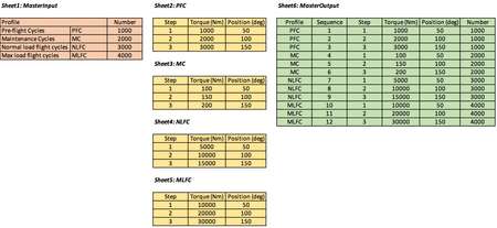
Hello, I want to create a dynamic table as shown in "sheet6". Sheet1 is the major overview with different load spectrums and number of occurrences. Sheet2-5 is specific load details for each spectrum, showing different load steps. Sheet6 take the table from sheet1 and add steps from sheet2-5. The column "number" in Sheet6 could be between profile and sequence. Order is not that important, just to show example. If anyone could help me to solve this, I would be very grateful! If possible, without using any code, just normal Excel functions. I'm thinking like a "lookup", where "Profile" in Sheet6 go to "Profile" in Sheet1, if match, extract complete table from sheet2-5 (depending of match). See overview below. Regards, Albin120Views0likes6Comments
Normalizing a text with numbers
Hello, i am looking for a fast ans simple (even VBA) solution to normalize text in a column. Let's say i have column B with values in the pattern A.9.1.1 What i want is every number to have two digits with a leading zero. It is easy to replace .1. with .01. with a vba macro in a loop. But the number at the end is difficult. I can not replace .1 with .01 as for example A.10.01.1 would become to A.010.1. You can see my problem? Of course i could loop through each cell value, grab the text after teh last dot an check if it is one or two digits. If it is one digit i can add the trailing zero. Is this the only way or ist there some secret function that will do this for me faster?Solved2.2KViews0likes7Comments
Excel & Word not working suspect temp folder error
My products are Microsoft Home & Student 2019 on Windows 11 Background: Yesterday accidently clicked on a link with the "screenconnect" virus. Was able to get it stopped before it downloaded on my computer. In attempting to stop it, I ran Microsoft virus check. I also went into Windows Privacy and Security and started Data Encryption, which I stopped after probably less than a minute and it did not complete. At some point received an error "make sure your temp folder is valid" NSIS error. Part of the NSIS error fix said to clear the temp folder, which I did. As a result of all the above, my Excel and Microsoft Word stopped working. I have tried all of the following fixes: Quick repair Complete repair Uninstalling program and reinstalling Recovered all the temp files from the recycle bin that were deleted and reloaded them into the temp file Checked Add-Ins in Excel - none are being used Made sure the temp folder is not set to read only Ran full virus scan Verified TEMP/TMP location Tried to find the folder "C:\users\"myname"\appdata\local\microsoft\windows\INetCache, but can't find INetCache file even when turning on hidden items Ran a complete disc check to check for disc errors In Excel, sometimes a document will open, other times it won't open at all and the program freezes. Even if I can open a document, I cannot modify it at all. I cannot create any new documents. When I attempt to create a new document, I get an error saying there isn't enough available memory or disc space (I have plenty of space on my hard drive). Prior to yesterday, I often had quite a few Excel files open at the same time. Also, all my templates disappeared before reinstalling the program. They reappeared when I reinstalled the program, but if I try and open them, an error says they are corrupted. Microsoft Word is also corrupted. These are some of the errors message I have received since reinstalling: Error writing temporary file. Make sure your temp folder is valid Microsoft Excel cannot access the file "C:\Users\"my name"\OneDrive\Documents\"file name". What should be the file name just appears as a number. The error message continues: "There are several possible reasons: - the file name or path does not exist. - the file is being used by another program. - the workbook you are trying to save has the same name as a currently open workbook" When trying to do a "save as" in Excel to try and create a new file get this error: C:\users\"myname"\onedrive\documents\"file name". File not found. Check the file name and try again "hardwareMonitorWindow: WINWORD.EXE - Application error: The exception unknown software exception (0xe00000002) occurred in the application at location....... then a big string of letters and numbers Microsoft Word: Word cannot save or create this file. Make sure that the disk you want to save the file on is not full, write-protected, or damaged." Microsoft Word: Word could not create the work file. Check the temp environment variable" I really don't know what to do at this point. Any help is appreciated. Thank you81Views0likes2Comments