Forum Discussion
TEXTJOIN formula that incorporates a look up?
Hello All,
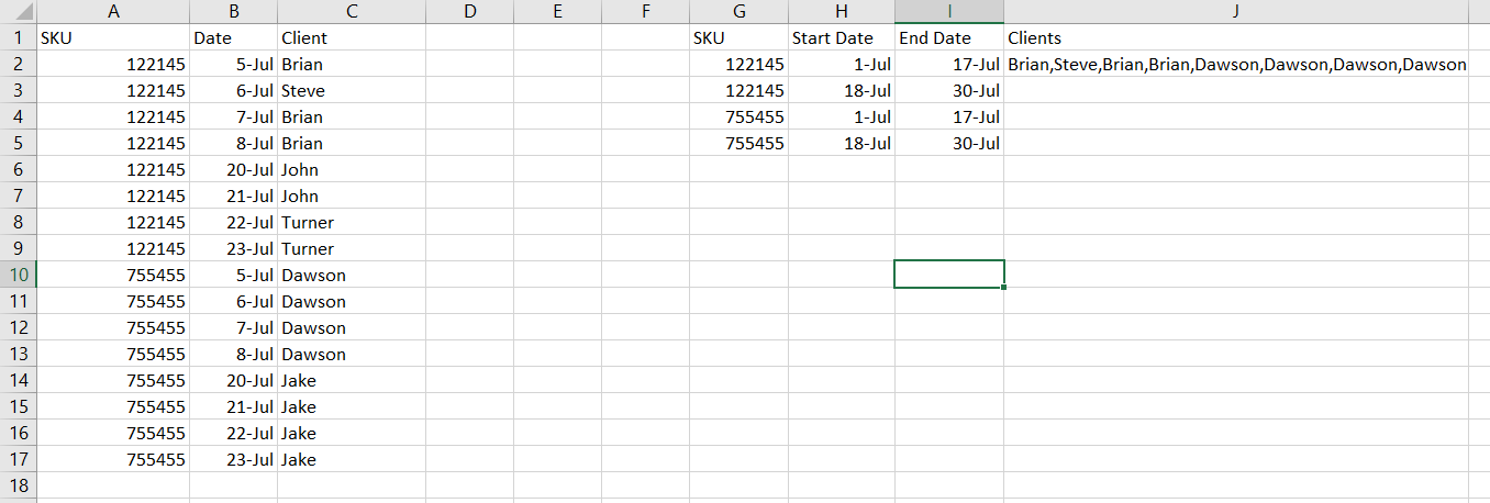
I have a scenario where for example : I have a list of SKU's for inventory in column A, Column B contains the date the SKU/Product was purchased. Column C lists the Client who purchased the SKU/Product. I need a formula that will look up the SKU and then return the names of the Clients which purchased the item within a set date range. For example between July 1st and July 17th for Product SKU 122145 It should return something like " Brian, Steve, Brian, Brian"
So Far I have
{=TEXTJOIN(",",1,IF(B:B>=H2,IF(B:B<=I2,C:C,""),""))}
Which returns : Brian,Steve,Brian,Brian,Dawson,Dawson,Dawson,Dawson
I want it to return only : Brian,Steve,Brian,Brian
As a Bonus if it could remove duplicates and return : Brian, Steve
that would be even better!
Thank you so much!
3 Replies
- SergeiBaklanDiamond Contributor
Hi Andrew,
That could be array formula
=TEXTJOIN(",",TRUE,IF(($B$2:$B$10>=$H2)*($B$2:$B$10<=$I2)*(MATCH($C$2:$C$10,$C$2:$C$10,0)=(ROW($C$2:$C$10)-ROW($C$1))),$C$2:$C$10,""))assuming you have no empty cells in Clients range.
Attached
 Andrew NhanCopper Contributor
Thank you SergeiBaklan!
This works great. However is there a way or a formula rather that will be able to look up the specific SKU in the list in column A and then return only the clients in the specific date range? For example in the formula you gave it works well if you sort filter column A in order and the select the specific data range of SKU 12214. However can we perform an extra step that looks up the SKU in G2 in Column A:A first and then proceed to the rest of the formula you listed?
- SergeiBaklanDiamond Contributor
Hi Andrew,
If SKU:s are not sorted perhaps this one will work
=TEXTJOIN(",",TRUE,IF(FREQUENCY(IF(($A$2:$A$10=$G2)*($B$2:$B$10>=$H2)*($B$2:$B$10<=$I2),MATCH($C$2:$C$10,$C$2:$C$10,0)),ROW($C$2:$C$10)-ROW($C$2)+1)>0,$C$2:$C$10,""))and attached